What problem does MPC-RL solve?
The repository junhengl/mpc-rl accompanies the paper Accelerating and Scaling MPC-Guided Reinforcement Learning for Humanoid Locomotion and Manipulation by Junheng Li, Liang Wu, Sergio A. Esteban, Lizhi Yang, Ján Drgoňa, and Aaron D. Ames. The paper appeared on arXiv on 2026-06-04 and asks a practical robotics question: can Model Predictive Control guide Reinforcement Learning during training, while the final deployed humanoid policy runs without MPC in the real-time loop?
That question matters because humanoid control sits between two imperfect tools. Pure RL can produce robust policies, but reward design is fragile. A velocity tracking reward may produce strange gaits. A foot slip penalty does not fully teach contact constraints. A standing reward does not tell the robot where its foot should land half a second later. MPC is the opposite: it has a dynamics model, explicit constraints, a prediction horizon, and physically meaningful contact forces. But online full-body MPC for a humanoid is expensive, especially when you need real-time deployment on hardware.
MPC-RL takes a pragmatic middle path:
- During training, a centroidal MPC runs in parallel for every environment.
- MPC generates references for CoM, linear momentum, angular momentum, ground reaction force, foot placement, and, for pushing, hand forces.
- Those references become reward terms and privileged critic inputs for PPO.
- During deployment, the actor sees only proprioception, command, and a phase clock. No MPC is required at inference time.
If you have read RL for Robotics: PPO, SAC and How to Choose Your Algorithm, think of MPC-RL as physics-structured reward shaping. If you already know Whole-Body MPC, the key difference is that MPC is not the runtime controller here. It is a training-time teacher.
Overall architecture
The paper calls this idea training-time MPC guidance. The diagram below from the repository shows the full loop: the simulator creates rollouts, MPC produces per-environment predictive references, the reward uses MPC landmarks, PPO updates actor and critic, and the final policy is exported without the MPC dependency.
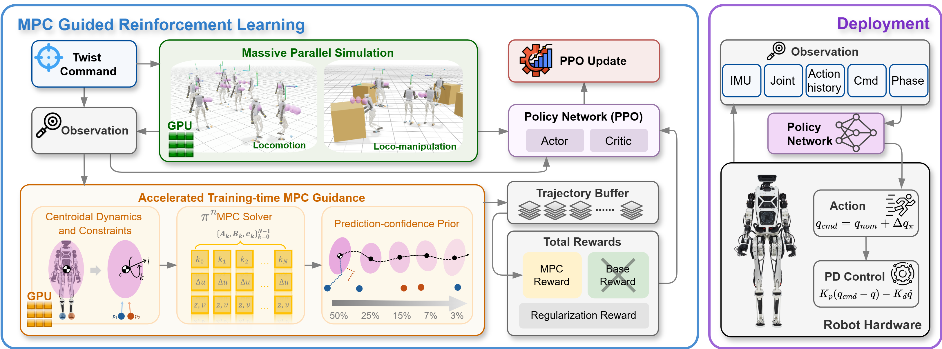
For a beginner, it helps to break the system into four blocks.
Block 1: Humanoid environment. The repo uses mjlab, MuJoCo, mujoco-warp, PyTorch, and rsl_rl. The target robot is the Westwood Robotics Themis V2 humanoid. The policy has 29 action dimensions. The action is not raw torque; it is a joint-position delta around a default pose, then tracked by per-joint PD controllers. This makes deployment easier because the neural policy outputs position offsets while low-level impedance handles stabilization.
Block 2: Centroidal Dynamics MPC. The MPC does not simulate the whole robot with every joint. It uses a 9-dimensional centroidal state:
xi = [ CoM position c,
       centroidal linear momentum l_G,
       centroidal angular momentum k_G ]
For locomotion, the MPC controls contact wrenches at the two feet. For loco-manipulation, it adds left-hand and right-hand pushing forces. This reduced model is far cheaper than full-body MPC but still captures the most important balance information: where the center of mass goes, how momentum changes, and whether contact forces respect friction and wrench constraints.
Block 3: π^n MPC solver. With 4096 parallel environments, running 4096 sequential MPC solvers would be impractical. The paper introduces π^n MPC, a batched GPU solver that parallelizes across both environments and the prediction horizon. It avoids repeatedly constructing large sparse QPs, operates directly on time-varying dynamics, and uses an ADMM-style variable splitting scheme so horizon updates can run in parallel.
Block 4: PPO policy. The actor observes deployable signals only: IMU angular velocity, projected gravity, joint positions and velocities, previous action, commanded velocity, and a phase clock sin(phi), cos(phi). The critic receives privileged information: base velocity, foot clearance, and MPC references. This is an asymmetric actor-critic setup. The critic gets richer training signals, while the actor stays hardware-ready.
MPC landmark reward: why not track only the next step?
A common mistake when using MPC as a teacher is to track only the next MPC output. That wastes the predictive part of MPC. The MPC already solves over a horizon, for example N = 10 with dt = 0.07 s, which means about 0.7 s of lookahead. If the policy only tracks the first point, it learns short-term reactions rather than long-horizon structure.
MPC-RL extracts a small set of landmarks from the full predicted trajectory. When the rollout reaches a time point, the realized CoM, CoM velocity, and angular momentum are compared against the landmarks that previous MPC solves predicted for that same time. The intuitive form is:
reward_mpc_com = exp(- sum_l alpha_l * error_l^2 / sigma^2)
alpha_l is a horizon-dependent weight. The paper uses a tapered schedule: near-term predictions receive higher weight, far-horizon predictions receive lower weight, with values like 0.5, 0.25, 0.15, 0.07, 0.03. This is sensible because near predictions are usually more reliable under model mismatch, while far predictions still provide useful direction.
For locomotion, the reward stack includes:
| Reward group | Meaning |
|---|---|
mpc_com |
Track MPC CoM landmarks |
mpc_lin_vel |
Track MPC CoM linear velocity |
mpc_ang_mom |
Regulate angular momentum against MPC |
mpc_foot |
Guide foot placement toward landing targets |
mpc_grf |
Softly align ground reaction forces with MPC |
| regularization | pose, gait, foot clearance, joint limit, self collision, action rate |
The important detail is that MPC rewards replace part of the base RL reward, such as velocity tracking and angular momentum regularization. They are not merely a small bonus on top. That makes the comparison between pure RL and MPC-RL cleaner: regularization stays shared, while the main driving signal changes.
π^n MPC: why the paper emphasizes scaling
Robot RL training usually uses thousands of environments. This repo trains with 4096 parallel environments by default. If each training update had to build a QP, compile symbolic expressions, or solve the horizon sequentially, MPC overhead would dominate the experiment.
The figure below from the repo compares GPU batch MPC/QP solvers as the number of environments and horizon length increase. The high-level takeaway is that π^n MPC remains practical for longer horizons, while several alternatives slow down sharply or run out of VRAM.
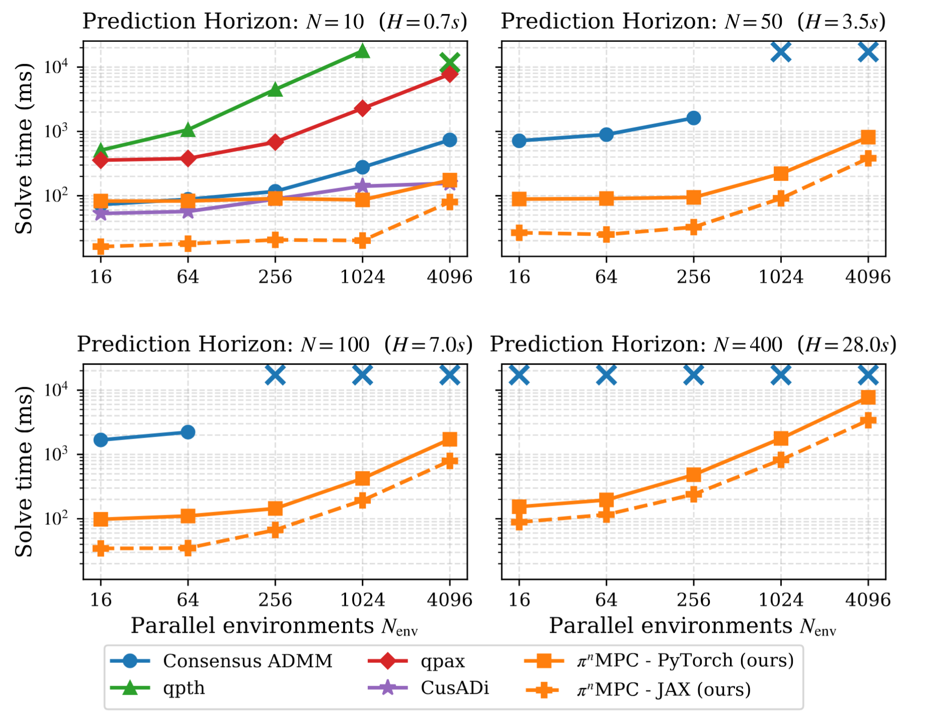
The paper compares against consensus ADMM, qpth, qpax, and CusADi. CusADi can have competitive solve speed in some settings, but the reported symbolic compilation for the MPC problem takes about 1.5 hours and requires substantial RAM. π^n MPC avoids that construction path. It exposes the prediction horizon as a batch dimension, uses standard batched GPU operations, and provides both JAX and PyTorch backends in the repository.
The simplest way to remember the difference is:
Pure online MPC:
  solve optimization at every robot control cycle during deployment

MPC-RL:
  solve many lightweight MPC problems during training
  convert MPC plans into reward and critic guidance
  deploy only the neural policy
This is very different from traditional MPC deployment. From a simulation-stack perspective, this repo relies on MuJoCo-Warp/mjlab to keep physics and GPU training tightly connected.
Repository setup
The repo requires Python 3.11 to 3.13 and a CUDA 12 GPU. The pyproject.toml pins several important dependencies:
| Package | Repo version | Role |
|---|---|---|
mjlab |
1.2.0 |
RL training framework and task registry |
mujoco |
3.6.0 |
Physics engine |
mujoco-warp |
3.6.0 |
GPU simulation stack |
warp-lang |
1.12.0 |
Warp backend compatible with mjlab |
torch |
2.10.0 |
PPO, tensors, PyTorch solver |
jax[cuda12] |
0.10.0 |
JAX backend for PiMPC |
The README setup is short:
git clone https://github.com/junhengl/mpc-rl
cd mpc-rl
uv sync
Before you run the default commands on your own workstation, check three things:
- Your NVIDIA driver supports CUDA 12.
uvis installed.- Your GPU has enough VRAM for the environment count you choose.
The paper reports experiments on an RTX 5090 with 32 GB of VRAM. If your GPU is smaller, reduce --env.scene.num-envs first. A beginner-friendly starting point is 512 or 1024 environments. Once the loop runs correctly, scale upward. Do not blindly copy 4096 before knowing your memory footprint.
Training locomotion
The locomotion task is:
Mjlab-MPC-Guided-Locomotion-Themis
The default training command is:
CUDA_VISIBLE_DEVICES=0 uv run train Mjlab-MPC-Guided-Locomotion-Themis \
  --env.scene.num-envs 4096 \
  --agent.max-iterations 15000
In the paper, physics is integrated at 200 Hz, the control rate is 50 Hz, and each episode lasts up to 20 s, or 1000 control steps. PPO uses separate actor and critic MLPs with hidden widths 512, 256, 128, ELU activations, a Gaussian action distribution, and a learnable scalar standard deviation.
The training workflow looks like this:
- The simulator creates 4096 copies of the environment.
- Each environment samples a velocity command.
- On the MPC schedule,
CentroidalMPCreads the current state, contact schedule, and command. - MPC solves a horizon and produces CoM, momentum, foot placement, and ground reaction force references.
- The reward manager computes terms such as
mpc_com,mpc_lin_vel,mpc_ang_mom,mpc_foot, andmpc_grf. - PPO updates the policy from rollouts.
- After many iterations, the actor learns to produce joint-position deltas that follow the structure of the MPC plan without calling MPC.
One beginner detail is easy to miss: run_every_n_steps. MPC does not need to solve at every physics step. With a 50 Hz control rate, the paper's default setting uses horizon N = 10 and a 10 Hz MPC update rate. That is frequent enough to guide learning, but not so frequent that training becomes unnecessarily expensive or the reward becomes overly rigid.
Training loco-manipulation
The second task is:
Mjlab-MPC-Guided-Loco-manipulation-Themis
The training command is:
CUDA_VISIBLE_DEVICES=0 uv run train Mjlab-MPC-Guided-Loco-manipulation-Themis \
  --env.scene.num-envs 4096 \
  --agent.max-iterations 25000
This task is walking while pushing a box. Compared with locomotion, the MPC includes hand-force variables. In LocoManipMPCConfig, the repo exposes parameters such as mu_hand, f_hand_max, R_f_hand, and R_hand_balance. The loco-manipulation MPC input also includes hand pose, hand contact gates, external body force and torque, and box resistance force.
That extra structure matters. Pure RL for pushing can suffer from poor exploration: the robot reaches the object but fails to maintain contact, pushes off-axis, or sacrifices balance to produce force. MPC-guided reward provides a physical hint: where the CoM should be while pushing, how momentum should evolve, how hand forces should balance, and how the feet should support the pushing direction.
The paper emphasizes that the loco-manipulation policy uses the same observation space as the locomotion policy and does not require object state at runtime like a pure MPC controller often would. This is useful for deployment. The robot does not need a perfect perception stack that estimates the box mass or full object state; it has already learned the pushing structure during training.
Resuming checkpoints and inference
The README gives this resume example:
CUDA_VISIBLE_DEVICES=0 uv run train Mjlab-MPC-Guided-Locomotion-Themis \
  --agent.resume True \
  --agent.load-run "2026-05-08_22-55-00" \
  --agent.load-checkpoint model_5000.pt
To play back a trained policy:
uv run play Mjlab-MPC-Guided-Locomotion-Themis --wandb-run-path <entity/project/run-id>
When moving from training to inference, remember the central design rule: MPC is only the teacher. The deployed actor needs deployable observations only:
actor_obs =
  IMU trunk angular velocity
  projected gravity
  joint positions relative to default
  joint velocities relative to default
  previous action
  velocity command
  phase clock
The critic and MPC references do not go onto the robot. If you port this idea to another humanoid, the parts that need the most care are the action interface, joint PD gains, sensor normalization, and phase/gait schedule. The paper also includes a section on choosing PD gains from effective inertia. Instead of using very stiff servo-like gains, the authors choose lower natural frequencies for Themis because its actuators have high inertia and low gear ratios. This avoids chatter at the hip and knee during hardware deployment.
Key results
The results have four main takeaways.
1. Better velocity tracking than pure RL. In the comparison table, pure RL reports RMSE vx = 0.1609, vy = 0.1566, and wz = 0.0912. The default MPC-RL setting, N = 10 at 10 Hz, reports vx = 0.1280, vy = 0.1326, and wz = 0.0928. The benefit is clearest in translational velocity tracking, including out-of-distribution commands whose bounds are 50% higher than the in-distribution commands.
2. Better push recovery in most directions. Pure RL tolerates different maximum pushes by direction, such as 300 N at 0 degrees, 100 N at 90 degrees, 350 N at 180 degrees, and 125 N at 270 degrees. The default MPC-RL configuration improves several directions: 375 N at 0 degrees, 125 N at 90 degrees, 450 N at 180 degrees, and other MPC-RL configurations reach stronger recovery at 270 degrees. The practical interpretation is that the policy learns a more structured contact and balance strategy, not just velocity command following.
3. Longer horizon is not always better. The paper tests N = 10, 30, and 50 at a 10 Hz update rate. The result is not monotonic. N = 10 is the best overall default. Longer horizons provide more lookahead, but they also increase model mismatch and reward delay. For Themis locomotion, roughly one gait-cycle lookahead is enough.
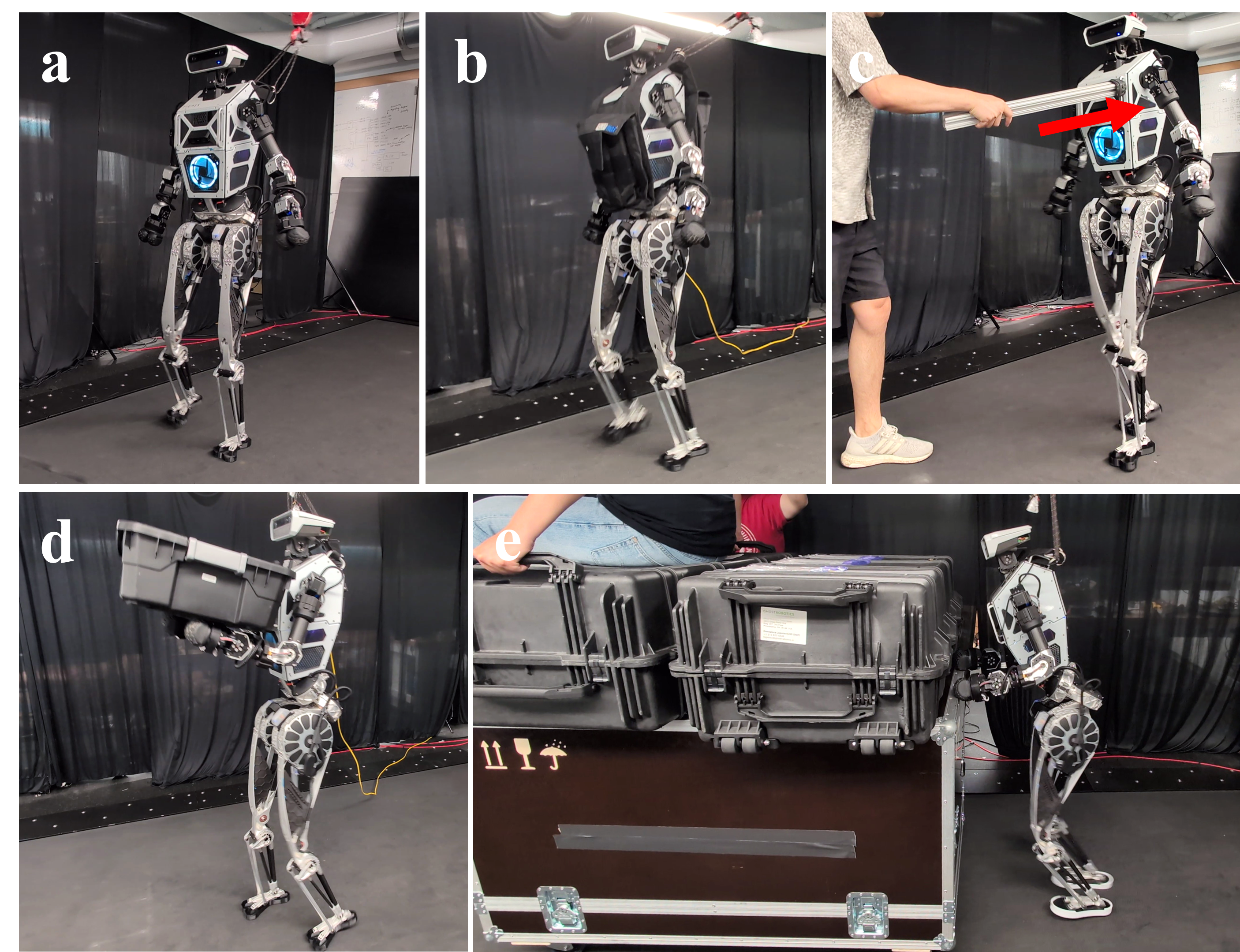
4. Loco-manipulation handles heavy pushing. In simulation, MPC-RL pushes a 20 kg, 1 m x 1 m x 1 m box with friction coefficient 0.2 and tracks velocity better than pure RL, which stalls from the start. On hardware, the robot pushes a cart payload up to 290 kg, or 829% of body mass, with a measured pushing force around 180 N. This is the most striking result because it shows that MPC guidance can help not only gait learning but also forceful whole-body contact manipulation.
How to read the repo
If you want to learn from the code rather than only run commands, read it in this order:
| File or folder | What to learn |
|---|---|
README.md |
task names, setup, training commands |
src/themis_mpc/centroidal_mpc.py |
MPCConfig, CentroidalMPC, foot contact constraints |
src/themis_mpc/loco_manip_mpc.py |
hand-force extension for pushing |
src/themis_training/mpc_grf_mdp.py |
how MPC runs as a command term in the environment |
src/themis_training/env_cfgs.py |
reward terms, observation noise, domain randomization |
pyproject.toml |
dependency versions and the mjlab.tasks entry point |
A beginner should first run play if the authors publish checkpoints, or reduce the environment count and test the training loop. Once the loop is stable, tune the MPC horizon, update rate, solver_type, and reward weights. If you are still building simulation foundations, learn basic MuJoCo workflow before going deep into the solver.
When should you use the MPC-RL idea?
MPC-RL is a good fit when three conditions hold:
- You have a reduced-order model that is good enough to provide guidance.
- Pure RL rewards struggle to encode contact, momentum, or long-horizon behavior.
- You do not want to run a heavy optimizer inside the real-time deployment loop.
It is not a silver bullet. If your simulator is inaccurate, the contact schedule is wrong, or the action interface is unstable, the MPC reward can teach the policy to follow an unsuitable teacher. The paper also lists limitations: centroidal dynamics is a reduced-order approximation, contact schedules are prescribed, and numerical solvers still have scaling limits. The authors point toward richer nonlinear MPC, more contact modes, and neural-network-augmented batch MPC solvers as future directions.
Even with those caveats, the contribution is clear: this repo turns MPC from a heavy online controller into a structured training signal. For humanoids, where reward design often decides whether a policy works at all, that pattern is worth learning.