Why MPC for Humanoids?
In Part 2, we learned about IK, operational space control, and QP-based whole-body control. But these methods are all reactive — they only look at current state to make decisions.
Model Predictive Control (MPC) is different: it looks into the future. MPC solves an optimization problem over a horizon (e.g., 0.5-1 second), calculates the best sequence of actions, executes the first step, then repeats. This is especially important for humanoids because:
- Contact planning: MPC can plan when to place feet, when to lift feet
- Balance recovery: Look ahead to prevent balance loss
- Whole-body coordination: Optimize locomotion and manipulation simultaneously
The most important recent paper: "Whole-Body Model-Predictive Control of Legged Robots with MuJoCo" (arXiv:2503.04613) — from John Z. Zhang (MIT), Taylor Howell, Yuval Tassa (Google DeepMind), and Guanya Shi (CMU). This paper proves MPC with MuJoCo can run real-time on real humanoids with zero-shot sim-to-real.

MPC — Basic Theory
Optimization Problem
MPC solves this problem at each timestep:
minimize: sum_{t=0}^{T-1} [ l(x_t, u_t) ] + l_T(x_T)
subject to:
    x_{t+1} = f(x_t, u_t)       (dynamics)
    x_0 = x_current              (initial state)
    u_min <= u_t <= u_max        (actuator limits)
    h(x_t, u_t) >= 0             (constraints: friction, joint limits, ...)
Where:
x_t— state (joint positions, velocities)u_t— control (joint torques or accelerations)f— dynamics modell— cost function (tracking error, energy, ...)T— prediction horizon (lookahead steps)
Receding Horizon
MPC repeats every control cycle (e.g., every 1-10 ms):
- Measure current state
x_0 - Solve optimization problem over horizon T
- Execute only
u_0(first step) - Return to step 1
This creates a natural feedback loop — if disturbed (e.g., pushed), MPC automatically adjusts the plan.
iLQR — Optimization Algorithm for MPC
iterative Linear Quadratic Regulator (iLQR) is the most commonly used algorithm for MPC on humanoids. It's the nonlinear version of LQR.
iLQR Algorithm — Iterative Linear Quadratic Regulator
iLQR approximates nonlinear problems by:
- Forward pass: Simulate trajectory with current control
- Backward pass: Linearize dynamics around trajectory, solve Riccati for feedback gains
- Forward pass: Update trajectory with new gains
- Repeat until convergence
The beauty of iLQR is that it naturally handles contact-implicit control — the forward simulation automatically computes contact dynamics (using MuJoCo's convex optimization solver), and the backward pass derives optimal gains that respect these constraints.
import numpy as np
import mujoco

class iLQR_MPC:
    def __init__(self, model, horizon=50, dt=0.01):
        self.model = model
        self.T = horizon
        self.dt = dt
        self.nx = model.nq + model.nv  # state dimension
        self.nu = model.nu              # control dimension

    def rollout(self, x0, U):
        """Forward simulate with control sequence U."""
        data = mujoco.MjData(self.model)
        X = [x0.copy()]

        for t in range(self.T):
            data.qpos[:] = X[-1][:self.model.nq]
            data.qvel[:] = X[-1][self.model.nq:]
            data.ctrl[:] = U[t]
            mujoco.mj_step(self.model, data)
            x_next = np.concatenate([data.qpos.copy(), data.qvel.copy()])
            X.append(x_next)

        return X

    def solve(self, x0, x_ref, U_init, Q, R, Qf, max_iter=10):
        """Run iLQR MPC."""
        self.x_ref = x_ref
        U = [u.copy() for u in U_init]

        for iteration in range(max_iter):
            # Forward rollout
            X = self.rollout(x0, U)

            # Compute cost
            cost = self._compute_cost(X, U, Q, R, Qf)

            # Update (simplified)
            if iteration > 0 and cost >= prev_cost:
                break  # Converged

            prev_cost = cost

        return U[0], X  # Return first control and trajectory

    def _compute_cost(self, X, U, Q, R, Qf):
        """Compute total cost."""
        cost = 0
        for t in range(self.T):
            x_err = X[t] - self.x_ref
            cost += x_err.T @ Q @ x_err
            cost += U[t].T @ R @ U[t]
        x_final_err = X[-1] - self.x_ref
        cost += x_final_err.T @ Qf @ x_final_err
        return cost
MuJoCo MPC — Official Implementation
Paper arXiv:2503.04613 uses MuJoCo as the dynamics model directly in the iLQR loop. Key features:
- Finite-difference derivatives: Instead of analytical derivatives (complex with contact), use finite differences on MuJoCo simulator. Fast because MuJoCo steps are very fast.
- Contact-implicit: No explicit contact schedule needed — MuJoCo automatically handles contact in forward simulation.
- Real-time: Achieves ~100 Hz control rate on real hardware (Unitree H1, quadrupeds).
Official code: github.com/johnzhang3/mujoco_mpc_deploy
Contact Dynamics — The Biggest Challenge
Contact (between feet and ground) is the hardest part of humanoid dynamics. Three states exist:
- No contact: Foot in air, no contact forces
- Sliding contact: Foot slides on ground, friction
- Sticking contact: Foot adheres to ground, static friction
Friction Cone
Contact forces are bounded by friction cone:
||f_tangential|| <= mu * f_normal
In MPC, the friction cone is approximated as a pyramid to convert it to linear constraints.

Real-Time Constraints
To run MPC real-time on humanoids (100-1000 Hz control loop):
1. Reduce Horizon
Instead of 100 steps, use 20-50 with larger timesteps. Trade-off: shorter look-ahead but less accuracy.
2. Warm-starting
Use the previous solution as starting point for the current one. Since state doesn't change much between cycles, warm-start helps converge faster (usually 1-3 iLQR iterations instead of 10+).
def mpc_loop(model, x0, x_ref, Q, R, Qf):
    """MPC loop with warm-starting."""
    T = 30  # horizon
    U_prev = [np.zeros(model.nu) for _ in range(T)]

    while True:
        x_current = get_state()  # Read from sensors

        # Warm-start: shift previous solution
        U_init = U_prev[1:] + [U_prev[-1]]

        # Solve MPC (only 2-3 iterations)
        mpc = iLQR_MPC(model, horizon=T)
        u_opt, K = mpc.solve(x_current, x_ref, U_init, Q, R, Qf, max_iter=3)

        # Apply control
        apply_torque(u_opt)

        # Save for next warm-start
        U_prev = U_init
3. GPU Acceleration
MuJoCo MJX (JAX backend) and MJX-Warp (NVIDIA GPU) run dynamics on GPU. Especially useful for sampling-based MPC (e.g., MPPI) — sample thousands of trajectories in parallel.
MPC vs QP vs RL
| Criterion | QP (Part 2) | MPC (iLQR) | RL (Part 4) |
|---|---|---|---|
| Look-ahead | No (reactive) | Yes (0.5-1s horizon) | Yes (learned) |
| Contact planning | Needs explicit schedule | Contact-implicit | Learned |
| Computation | ~1 ms | ~5-50 ms | ~0.1 ms (inference) |
| Robustness | Medium | Good (replans) | Best |
| Domain transfer | Good (model-based) | Good (model-based) | Needs sim-to-real |
| Dexterity | Good | Good | Best |
| Setup effort | Medium | High | High (training) |
Hybrid MPC + RL
Latest trend: combine both:
- RL learns rough policy (robust, fast)
- MPC refines real-time (precise, optimal)
Example: RL for locomotion, MPC for fine manipulation. Or RL provides warm-start for MPC.
Learning Resources
- Code: github.com/johnzhang3/mujoco_mpc_deploy — Real-world MPC deployment
- Paper: arXiv:2503.04613 — Whole-Body MPC with MuJoCo
- MuJoCo MPC: github.com/google-deepmind/mujoco_mpc — Official framework
- Tutorial: REx Lab project page
Next in This Series
- Part 2: Humanoid Control Basics: IK to Task-Space Control
- Part 4: RL for Humanoid: From Humanoid-Gym to Sim2Real — Reinforcement learning approach
- Part 5: Loco-Manipulation: Walking and Manipulating Together
Related Articles
- Simulation for Robotics: MuJoCo vs Isaac Sim vs Gazebo — Simulator comparison
- Getting Started with MuJoCo — Hands-on MuJoCo tutorial
- RL for Bipedal Walking — RL for two-legged robots
- Sim-to-Real Transfer — Moving from simulation to real hardware