Tại sao MPC cho Humanoid?
Trong Part 2, chúng ta đã học về IK, operational space control, và QP-based whole-body control. Nhưng các phương pháp đó đều là reactive -- chỉ nhìn vào trạng thái hiện tại để ra quyết định.
Model Predictive Control (MPC) khác biệt ở chỗ: nó nhìn trước tương lai. MPC giải bài toán tối ưu trên một horizon (ví dụ 0,5-1 giây), tính toán chuỗi hành động tốt nhất, thực hiện bước đầu tiên, rồi lặp lại. Điều này đặc biệt quan trọng cho humanoid vì:
- Contact planning: MPC có thể lên kế hoạch khi nào đặt chân, khi nào nhấc chân
- Balance recovery: Nhìn trước để phòng tình huống mất thăng bằng
- Whole-body coordination: Tối ưu đồng thời locomotion và manipulation
Paper quan trọng nhất gần đây: "Whole-Body Model-Predictive Control of Legged Robots with MuJoCo" (arXiv:2503.04613) -- từ John Z. Zhang (MIT), Taylor Howell, Yuval Tassa (Google DeepMind), và Guanya Shi (CMU). Paper này chứng minh MPC với MuJoCo có thể chạy real-time trên humanoid thật với zero-shot sim-to-real.

MPC -- Lý thuyết cơ bản
Bài toán tối ưu
MPC giải bài toán sau tại mỗi thời điểm:
minimize: sum_{t=0}^{T-1} [ l(x_t, u_t) ] + l_T(x_T)
subject to:
    x_{t+1} = f(x_t, u_t)       (dynamics)
    x_0 = x_current              (initial state)
    u_min <= u_t <= u_max        (actuator limits)
    h(x_t, u_t) >= 0             (constraints: friction, joint limits, ...)
Trong đó:
x_t-- trạng thái (joint positions, velocities)u_t-- điều khiển (joint torques hoặc accelerations)f-- mô hình động lực học (dynamics model)l-- cost function (tracking error, energy, ...)T-- prediction horizon (số bước nhìn trước)
Receding Horizon
MPC lặp lại mỗi control cycle (ví dụ mỗi 1-10 ms):
- Đo trạng thái hiện tại
x_0 - Giải bài toán tối ưu trên horizon T
- Thực hiện chỉ
u_0(bước đầu tiên) - Quay lại bước 1
Điều này tạo ra feedback loop tự nhiên -- nếu có nhiễu loạn (ví dụ bị đẩy), MPC sẽ tự động điều chỉnh kế hoạch.
iLQR -- Thuật toán tối ưu cho MPC
iterative Linear Quadratic Regulator (iLQR) là thuật toán được dùng nhiều nhất cho MPC trên humanoid. Nó là phiên bản nonlinear của LQR.
LQR recap
LQR giải bài toán với dynamics tuyến tính và cost bậc 2:
dynamics: x_{t+1} = A*x_t + B*u_t
cost: x^T*Q*x + u^T*R*u
Nghiệm tối ưu là feedback gain: u = -K*x, tính bằng Riccati equation.
iLQR -- Mở rộng cho nonlinear
iLQR xấp xỉ bài toán nonlinear bằng cách:
- Forward pass: Simulate trajectory với control hiện tại
- Backward pass: Tuyến tính hóa dynamics quanh trajectory, giải Riccati để tìm feedback gains
- Forward pass: Cập nhật trajectory với gains mới
- Lặp lại đến hội tụ
import numpy as np
import mujoco

class iLQR_MPC:
    def __init__(self, model, horizon=50, dt=0.01):
        self.model = model
        self.T = horizon
        self.dt = dt
        self.nx = model.nq + model.nv  # state dimension
        self.nu = model.nu              # control dimension

    def rollout(self, x0, U):
        """Forward simulate với chuỗi control U."""
        data = mujoco.MjData(self.model)
        X = [x0.copy()]

        for t in range(self.T):
            # Set state
            data.qpos[:] = X[-1][:self.model.nq]
            data.qvel[:] = X[-1][self.model.nq:]
            data.ctrl[:] = U[t]

            # Step
            mujoco.mj_step(self.model, data)

            x_next = np.concatenate([data.qpos.copy(), data.qvel.copy()])
            X.append(x_next)

        return X

    def linearize(self, x, u, eps=1e-6):
        """Tính A, B matrices bằng finite differences."""
        data = mujoco.MjData(self.model)

        # Nominal next state
        data.qpos[:] = x[:self.model.nq]
        data.qvel[:] = x[self.model.nq:]
        data.ctrl[:] = u
        mujoco.mj_step(self.model, data)
        x_nom = np.concatenate([data.qpos.copy(), data.qvel.copy()])

        # A = df/dx (finite differences)
        A = np.zeros((self.nx, self.nx))
        for i in range(self.nx):
            x_plus = x.copy()
            x_plus[i] += eps

            data.qpos[:] = x_plus[:self.model.nq]
            data.qvel[:] = x_plus[self.model.nq:]
            data.ctrl[:] = u
            mujoco.mj_step(self.model, data)
            x_next_plus = np.concatenate([data.qpos.copy(), data.qvel.copy()])

            A[:, i] = (x_next_plus - x_nom) / eps

        # B = df/du (finite differences)
        B = np.zeros((self.nx, self.nu))
        for i in range(self.nu):
            u_plus = u.copy()
            u_plus[i] += eps

            data.qpos[:] = x[:self.model.nq]
            data.qvel[:] = x[self.model.nq:]
            data.ctrl[:] = u_plus
            mujoco.mj_step(self.model, data)
            x_next_plus = np.concatenate([data.qpos.copy(), data.qvel.copy()])

            B[:, i] = (x_next_plus - x_nom) / eps

        return A, B

    def backward_pass(self, X, U, Q, R, Qf):
        """Backward pass: tính feedback gains K và feedforward k."""
        K_list = []
        k_list = []

        # Terminal cost gradient
        Vx = Qf @ (X[-1] - self.x_ref)
        Vxx = Qf.copy()

        for t in reversed(range(self.T)):
            A, B = self.linearize(X[t], U[t])

            # Cost gradients
            lx = Q @ (X[t] - self.x_ref)
            lu = R @ U[t]

            # Q-function
            Qx = lx + A.T @ Vx
            Qu = lu + B.T @ Vx
            Qxx = Q + A.T @ Vxx @ A
            Quu = R + B.T @ Vxx @ B
            Qux = B.T @ Vxx @ A

            # Regularization
            Quu_reg = Quu + 1e-6 * np.eye(self.nu)

            # Gains
            K = -np.linalg.solve(Quu_reg, Qux)
            k = -np.linalg.solve(Quu_reg, Qu)

            # Update value function
            Vx = Qx + K.T @ Quu @ k + K.T @ Qu + Qux.T @ k
            Vxx = Qxx + K.T @ Quu @ K + K.T @ Qux + Qux.T @ K

            K_list.insert(0, K)
            k_list.insert(0, k)

        return K_list, k_list

    def solve(self, x0, x_ref, U_init, Q, R, Qf, max_iter=10):
        """Chạy iLQR MPC."""
        self.x_ref = x_ref
        U = [u.copy() for u in U_init]

        for iteration in range(max_iter):
            # Forward rollout
            X = self.rollout(x0, U)

            # Backward pass
            K_list, k_list = self.backward_pass(X, U, Q, R, Qf)

            # Forward pass với line search
            alpha = 1.0
            for _ in range(10):
                U_new = []
                X_new = [x0.copy()]

                for t in range(self.T):
                    dx = X_new[-1] - X[t]
                    u_new = U[t] + alpha * k_list[t] + K_list[t] @ dx
                    U_new.append(u_new)
                    X_new = self.rollout(x0, U_new)  # Simplified
                    break  # Simplified

                U = U_new
                break

        return U[0], K_list[0]  # Trả về control và gain đầu tiên
MuJoCo MPC -- Implementation chính thức
Paper arXiv:2503.04613 sử dụng MuJoCo làm dynamics model trực tiếp trong iLQR loop. Điểm đặc biệt:
- Finite-difference derivatives: Thay vì analytical derivatives (phức tạp với contact), dùng finite differences trên MuJoCo simulator. Nhanh vì MuJoCo step rất nhanh.
- Contact-implicit: Không cần explicit contact schedule -- MuJoCo tự động xử lý contact trong forward simulation.
- Real-time: Đạt ~100 Hz control rate trên hardware thật (Unitree H1, quadruped).
Code chính thức: github.com/johnzhang3/mujoco_mpc_deploy
Contact Dynamics -- Thách thức lớn nhất
Contact (tiếp xúc giữa chân và mặt đất) là phần khó nhất của humanoid dynamics. Có 3 trạng thái:
- No contact: Chân ở trên không, không có lực tiếp xúc
- Sliding contact: Chân trượt trên mặt đất, lực ma sát
- Sticking contact: Chân dính trên mặt đất, static friction
Complementarity constraints
Contact được mô hình hóa bằng complementarity conditions:
f_n >= 0           (lực pháp tuyến không âm)
phi >= 0           (không xâm nhập)
f_n * phi = 0      (hoặc không tiếp xúc, hoặc lực = 0)
MuJoCo giải contact bằng convex optimization -- chính xác và ổn định hơn impulse-based methods (dùng trong Gazebo/ODE).
Friction cone
Lực ma sát bị giới hạn bởi friction cone:
||f_t|| <= mu * f_n
Trong MPC, friction cone thường được xấp xỉ bằng pyramid để chuyển về linear constraint.

Real-Time Constraints
Để chạy MPC real-time trên humanoid (100-1000 Hz control loop), cần:
1. Giảm horizon
Thay vì 100 bước, dùng 20-50 bước với timestep lớn hơn. Trade-off: nhìn xa hơn nhưng ít chính xác hơn.
2. Warm-starting
Dùng nghiệm của lần trước làm điểm bắt đầu cho lần này. Vì trạng thái không thay đổi nhiều giữa 2 control cycles, warm-start giúp hội tụ nhanh hơn (thường 1-3 iLQR iterations thay vì 10+).
def mpc_loop(model, x0, x_ref, Q, R, Qf):
    """MPC loop với warm-starting."""
    T = 30  # horizon
    U_prev = [np.zeros(model.nu) for _ in range(T)]

    while True:
        x_current = get_state()  # Đọc từ sensors

        # Warm-start: shift previous solution
        U_init = U_prev[1:] + [U_prev[-1]]

        # Solve MPC (chỉ 2-3 iterations)
        mpc = iLQR_MPC(model, horizon=T)
        u_opt, K = mpc.solve(x_current, x_ref, U_init, Q, R, Qf, max_iter=3)

        # Apply control
        apply_torque(u_opt)

        # Lưu cho warm-start lần sau
        U_prev = U_init
3. Parallel computation
Linearization (tính A, B) tại mỗi thời điểm có thể chạy song song. MuJoCo thread-safe, nên có thể dùng multi-threading.
4. GPU acceleration
MuJoCo MJX (JAX backend) và MJX-Warp (NVIDIA GPU) cho phép chạy dynamics trên GPU. Đặc biệt hữu ích cho sampling-based MPC (ví dụ MPPI) -- sample hàng nghìn trajectories song song.
MPC vs QP vs RL
| Tiêu chí | QP (Part 2) | MPC (iLQR) | RL (Part 4) |
|---|---|---|---|
| Nhìn trước | Không (reactive) | Có (0,5-1s horizon) | Có (learned) |
| Contact planning | Cần explicit schedule | Contact-implicit | Learned |
| Computation | ~1 ms | ~5-50 ms | ~0,1 ms (inference) |
| Robustness | Trung bình | Khá (replan) | Tốt nhất |
| Domain transfer | Tốt (model-based) | Tốt (model-based) | Cần sim-to-real |
| Dexterity | Tốt | Tốt | Tốt nhất |
| Setup effort | Trung bình | Cao | Cao (training) |
Kết hợp MPC + RL
Xu hướng mới nhất là kết hợp cả hai:
- RL học policy thô (robust, fast)
- MPC tinh chỉnh real-time (precise, optimal)
Ví dụ: RL policy cho locomotion, MPC cho manipulation tinh vi. Hoặc RL cung cấp warm-start cho MPC.
Paper arXiv:2408.00342 -- "MuJoCo MPC for Humanoid Control" -- so sánh chi tiết MPC và RL trên HumanoidBench.
Thực hành: MuJoCo MPC cho Humanoid Walking
import mujoco
import mujoco.viewer
import numpy as np

# Load humanoid model
model = mujoco.MjModel.from_xml_path("humanoid.xml")
data = mujoco.MjData(model)

# MPC parameters
horizon = 30
dt = 0.01
Q_pos = 10.0 * np.eye(model.nq)    # Position tracking weight
Q_vel = 1.0 * np.eye(model.nv)     # Velocity tracking weight
R_ctrl = 0.01 * np.eye(model.nu)   # Control effort weight
Q = np.block([[Q_pos, np.zeros((model.nq, model.nv))],
              [np.zeros((model.nv, model.nq)), Q_vel]])
Qf = 10.0 * Q  # Terminal cost

# Target: đi thẳng 0,5 m/s
x_ref = np.zeros(model.nq + model.nv)
x_ref[0] = 1.0  # Target x position (1m ahead)

# Initialize MPC
mpc = iLQR_MPC(model, horizon=horizon, dt=dt)
U_init = [np.zeros(model.nu) for _ in range(horizon)]

# Run
with mujoco.viewer.launch_passive(model, data) as viewer:
    while viewer.is_running():
        x_current = np.concatenate([data.qpos.copy(), data.qvel.copy()])

        # Solve MPC
        u_opt, K = mpc.solve(x_current, x_ref, U_init, Q, R_ctrl, Qf, max_iter=3)

        # Apply
        data.ctrl[:] = u_opt
        mujoco.mj_step(model, data)
        viewer.sync()
Tài nguyên học thêm
- Code: github.com/johnzhang3/mujoco_mpc_deploy -- Real-world MPC deployment
- Paper: arXiv:2503.04613 -- Whole-Body MPC with MuJoCo
- MuJoCo MPC: github.com/google-deepmind/mujoco_mpc -- Official MuJoCo MPC framework
- Tutorial: REx Lab project page
Tiếp theo trong series
- Part 2: Humanoid control cơ bản: IK đến task-space control
- Part 4: RL cho Humanoid: Humanoid-Gym đến sim2real -- Reinforcement learning approach
- Part 5: Loco-Manipulation: Robot vừa đi vừa thao tác
Bài viết liên quan
- Simulation cho Robotics: MuJoCo vs Isaac Sim vs Gazebo -- So sánh simulator
- Bắt đầu với MuJoCo -- Hands-on MuJoCo tutorial
- RL cho Bipedal Walking -- RL cho robot đi 2 chân
- Sim-to-Real Transfer -- Chuyển từ simulation sang thực tế