By the end of Part 4, our vehicle knew two things: where it is, to roughly 1.6 cm of lateral error, and what surrounds it — other vehicles, pedestrians, lane markings, traffic lights. But knowing is not driving. The next question is the hardest one in the entire stack: what should it do now?
This is the part newcomers underestimate. Perception has leaderboards, mAP scores, and public datasets — right and wrong are measurable on the spot. Planning does not work that way: a trajectory that looks correct on paper can still make passengers carsick, force the car behind into a hard brake, or leave the vehicle stranded at a busy roundabout because it is too polite to merge. And as the last section of this article shows, planning is also the layer where deep learning has still not beaten hand-written rules on the most serious closed-loop benchmark available in 2026.
Series roadmap
- Part 1 — SAE Level 2 vs 2+ vs 3 vs 4: who is responsible for driving, ODD and fallback.
- Part 2 — Sensor fusion: camera, radar and LiDAR building perception that degrades safely.
- Part 3 — Perception: 3D detection, occupancy grids and tracking on nuScenes.
- Part 4 — Localization and HD maps: GNSS/IMU fusion, NDT on LiDAR, map-free approaches.
- Part 5 — Planning and control: from rule-based to MPC and PDM, tracking a real trajectory.
- Part 6 — Validation: ISO 26262, SOTIF and Euro NCAP — proving safety without driving the miles.
Four decision layers — and why they must be separated
Nobody writes a single function that takes a point cloud and returns a steering angle. The problem is split into four layers, each with a horizon and a rate that differ by orders of magnitude:
| Layer | Question answered | Horizon | Rate | Typical tooling |
|---|---|---|---|---|
| Route / mission | Which roads lead to the destination? | 1–50 km | 0.1–1 Hz | Dijkstra/A* on a Lanelet2 routing graph |
| Behavior | Follow the lane, change lanes, or yield? | 5–15 s | 5–10 Hz | FSM, behavior tree, scenario manager |
| Motion / local | What is the concrete (x, y, v, t) trajectory? | 3–8 s | 10–20 Hz | Frenet lattice, optimization, MPC |
| Control | How many degrees of steering, how much throttle? | 0.5–2 s | 50–100 Hz | PID, pure pursuit, Stanley, LQR, MPC |
The reason for the split is not architectural elegance — it is the compute budget. A nonlinear optimizer running over a 30-second horizon with every dynamic obstacle modeled will never close a 100 Hz loop. Split the problem and each layer solves something that fits the time it actually has.
Notice that every layer consumes the output of Part 4 directly. Routing runs on Lanelet2 topology, the motion planner uses the lane centerline as its reference axis, and the controller needs centimeter-grade pose to know how far off it is.
Layer 1 — Route planning on the Lanelet2 routing graph
Lanelet2 is not only geometry: it can build a routing graph where each lanelet is a node and edges encode "you may continue here", "you may change left", "you may change right". Route finding becomes a classic graph problem.
import lanelet2
from lanelet2.projection import UtmProjector
from lanelet2.io import Origin

# Load a Lanelet2 map (OSM XML format)
projector = UtmProjector(Origin(21.0278, 105.8342))   # map origin
lmap = lanelet2.io.load("map.osm", projector)

# Traffic rules: right-hand traffic, passenger vehicle
traffic_rules = lanelet2.traffic_rules.create(
    lanelet2.traffic_rules.Locations.Germany,
    lanelet2.traffic_rules.Participants.Vehicle,
)
graph = lanelet2.routing.RoutingGraph(lmap, traffic_rules)

start = lmap.laneletLayer[1001]
goal = lmap.laneletLayer[2042]

# withLaneChanges=True: allow solutions that require changing lanes
route = graph.getRoute(start, goal, 0, withLaneChanges=True)
if route is None:
    raise RuntimeError("No valid route exists within the map's ODD")

path = route.shortestPath()
print(f"Lanelets on route: {len(path)}")
print(f"Route length: {route.length2d():.1f} m")
An easily missed detail: lane changes are not free. If you set the lane-change cost to plain geometric length, the planner will happily return a route demanding three lane changes in 80 m — topologically valid, kinematically impossible. Autoware handles this with an explicit penalty factor plus a minimum required distance for each lane change before the next turn.
Layer 2 — Behavior planning and the limits of rules
The behavior planner takes the route and decides the current driving mode. The most common implementation is still a finite state machine:
from enum import Enum

class Behavior(Enum):
    LANE_FOLLOW      = "lane following"
    LANE_CHANGE_LEFT = "changing left"
    PREPARE_CHANGE   = "preparing to change"
    STOP_AT_LINE     = "stopping at line"
    YIELD_CROSSING   = "yielding at crossing"

def decide(state, ego, scene):
    """Return the next behavior. Check order IS priority order."""
    # 1. Safety first: a red light or stop line beats every other intention
    if scene.stop_line_ahead_m < ego.braking_distance_m():
        return Behavior.STOP_AT_LINE
    # 2. Pedestrian in or entering the crossing
    if scene.pedestrian_at_crossing:
        return Behavior.YIELD_CROSSING
    # 3. Route demand: how far until we must be in the left lane to turn
    if scene.distance_to_required_change_m < 200:
        if scene.left_gap_s > 3.0 and scene.left_gap_ahead_s > 1.5:
            return Behavior.LANE_CHANGE_LEFT
        return Behavior.PREPARE_CHANGE   # slow down, indicate, wait for a gap
    return Behavior.LANE_FOLLOW
That code looks harmless, which is exactly the trap. With 5 behaviors there are 20 transition pairs to reason about. With 15 behaviors — a realistic number for an urban stack — there are 210. Both Apollo and Autoware abandoned the flat FSM: Apollo moved to a scenario–stage architecture (each scenario such as "unsignalized intersection" or "parallel parking" is its own sub-state-machine), while Autoware runs behavior_path_planner as priority-ordered modules executed in parallel and merged afterwards.
The general lesson transfers well beyond driving: once the rule count exceeds what a person can hold in their head, the fix is not more rules but a structure in which rules stop interacting pairwise.
Layer 3 — Motion planning in the Frenet frame
This is where the HD map pays a dividend. Instead of planning in Cartesian (x, y) — where "go straight" along a curved road is an awkward function — we switch to a Frenet frame anchored on the lanelet centerline:
s: arc length along the centerlined: lateral offset from the centerline
In this frame, "keep the lane" is simply d ≈ 0, and "change left" is d moving from 0 to +3.5. Road curvature disappears from the problem statement.
The Frenet optimal trajectory algorithm (Werling et al., ICRA 2010) generates a forest of candidates by sampling: for each pair of (target lateral offset d_T, time to target T), it connects the current and target states with a quintic polynomial for d(t) and a quartic for s(t). Why quintic? Because six boundary conditions must be matched — position, velocity, and acceleration at both ends — and a quintic is the lowest order with six free coefficients. A useful side effect: that solution minimizes jerk, which is exactly what passengers feel.
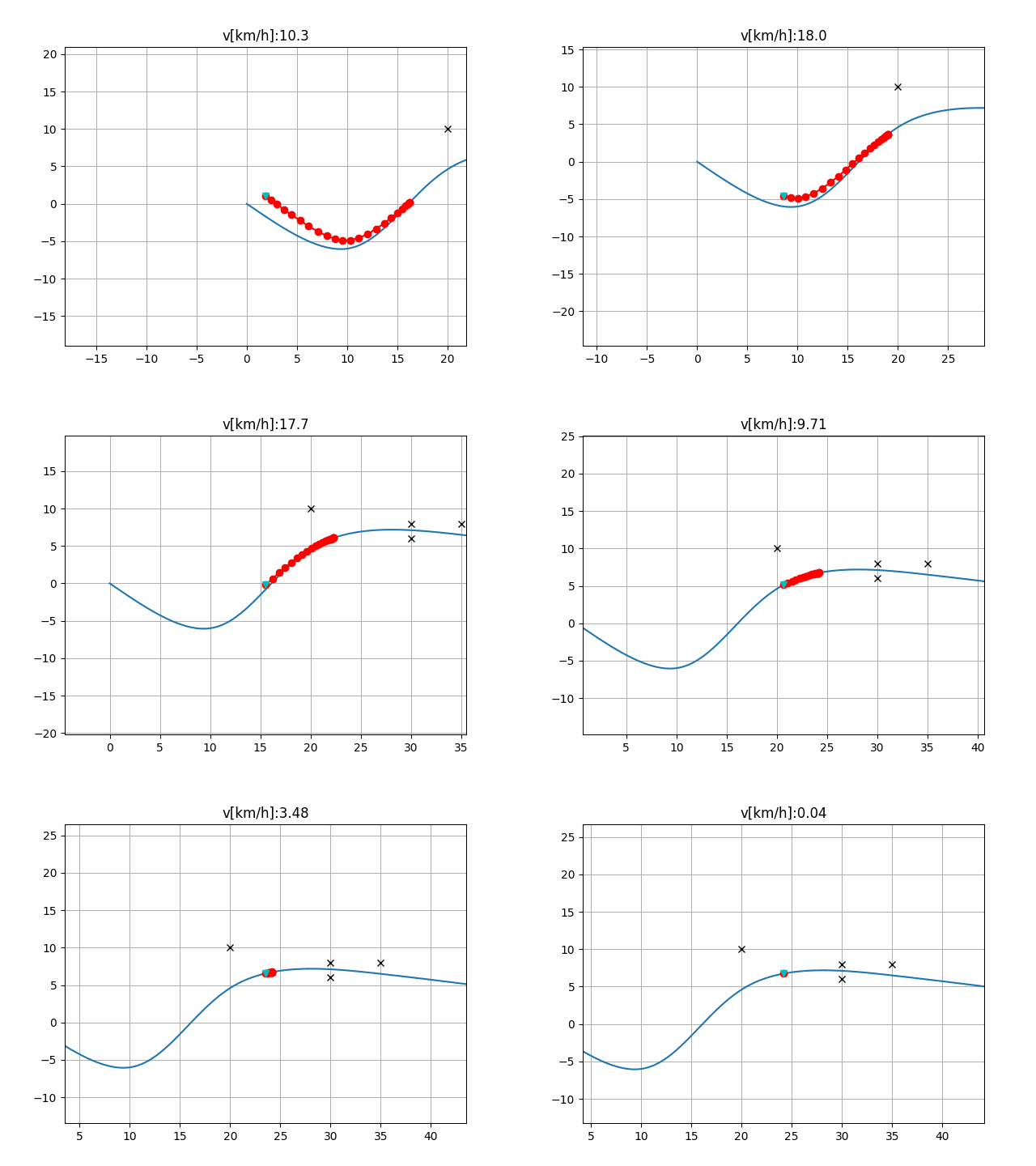
Frenet optimal trajectory at high speed with merging and stopping: thin lines are rejected candidates (collision or kinematic limit violation), the bold line is the selected trajectory. Source: AtsushiSakai/PythonRoboticsGifs repo
A typical cost function per candidate:
J = k_j · ∫ jerk² dt + k_T · T + k_d · d_T² + k_v · (v_T − v_target)²
Those four terms are the four things we are balancing: comfort, progress, lane centering, and desired speed. Every candidate must then survive three hard filters — exceeding the acceleration envelope, exceeding steering curvature, or colliding with the predicted trajectory of any tracked object (from the tracking module in Part 3).
A subtlety beginners miss: the planner does not check collisions against the current position of other vehicles, but against their predicted position at the matching time along the trajectory. Checking the former is the most reliable way to build a car that slams the brakes at every vehicle crossing in front of it.
Layer 4 — Control: four rungs from geometry to optimization
Pure pursuit — pure geometry
Pick a point on the trajectory at a lookahead distance L_d, then compute the steering angle for the circular arc connecting the vehicle to that point:
δ = arctan( 2·L·sin(α) / L_d )
where L is the wheelbase and α is the angle between the vehicle heading and the bearing to the lookahead point. Typically L_d = k·v + L_min, so the car looks further ahead at speed.
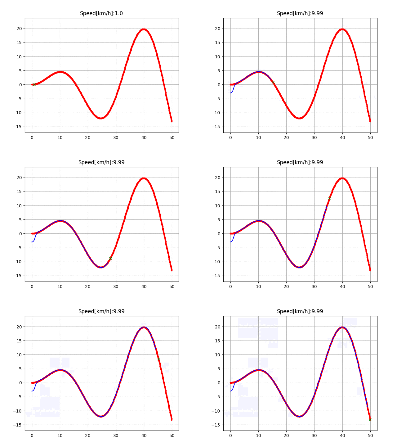
Pure pursuit: the lookahead point slides along the trajectory and the vehicle always follows the arc that reaches it. Source: AtsushiSakai/PythonRoboticsGifs repo
Upside: two lines of code and no vehicle model required. Downside: it always cuts corners on tight curves, and L_d is a knob that must be hand-tuned per speed band.
Stanley — correcting heading and cross-track error together
Stanley (born on the vehicle that won the 2005 DARPA Grand Challenge) sums two terms: heading error and speed-normalized cross-track error.
δ = (ψ_path − ψ_ego) + arctan( k·e_fa / (v + k_soft) )
The important difference from pure pursuit: Stanley measures error at the front axle rather than the center of gravity, which makes it track edges considerably better at low speed.
LQR — a model enters the picture
LQR linearizes the error dynamics around the reference trajectory, then solves the Riccati equation for the gain matrix K that is optimal for the quadratic cost ∫(xᵀQx + uᵀRu)dt. Changing Q and R trades tracking tightness against steering smoothness in a principled way rather than by feel.
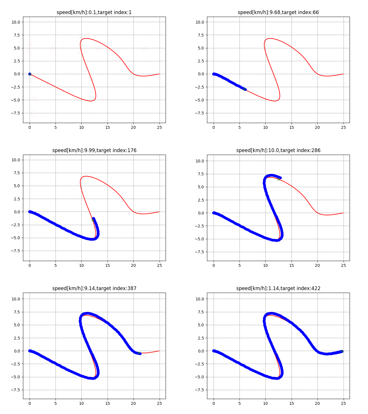
LQR speed and steering control: the optimal gain is recomputed for the current speed, driving the longitudinal and lateral axes together. Source: AtsushiSakai/PythonRoboticsGifs repo
MPC — looking ahead and respecting constraints
All three methods above share a weakness: they react rather than anticipate, and none of them can express a constraint like "steering angle must stay under 30 degrees" or "steering rate must stay under 200 deg/s". MPC solves precisely that: each cycle it optimizes over an N-step horizon, applies only the first control step, and repeats next cycle (receding horizon).
Here is a working lane-keeping MPC built on the linearized lateral-error bicycle model in the Frenet frame — pip install cvxpy numpy and it runs:
import numpy as np
import cvxpy as cp

# --- Vehicle and controller parameters ---
L    = 2.7      # wheelbase (m)
DT   = 0.05     # 20 Hz control cycle
N    = 20       # 20-step horizon = 1.0 s
V    = 15.0     # longitudinal speed (m/s), held constant over the next second

DELTA_MAX  = np.deg2rad(30.0)          # mechanical steering limit
DRATE_MAX  = np.deg2rad(200.0) * DT    # steering rate limit per step

# Lateral error model: x = [e_y, e_psi]
#   e_y'   = V * e_psi
#   e_psi' = (V / L) * delta  -  V * kappa_ref   (kappa_ref = reference curvature)
A = np.array([[1.0, V * DT],
              [0.0, 1.0]])
B = np.array([[0.0],
              [V * DT / L]])
E = np.array([[0.0],
              [-V * DT]])          # measured-disturbance matrix (curvature feedforward)

Q  = np.diag([10.0, 1.0])   # penalize lateral error more than heading error
Qf = np.diag([50.0, 5.0])   # heavier penalty on the terminal state
R  = np.array([[1.0]])      # penalize steering magnitude
Rd = np.array([[50.0]])     # penalize steering change — this is what makes it smooth

def solve_mpc(x0, kappa_ref, delta_prev):
    """x0: current [e_y, e_psi]. kappa_ref: N-step curvature profile (1/m)."""
    x = cp.Variable((2, N + 1))
    u = cp.Variable((1, N))

    cost = 0.0
    constraints = [x[:, 0] == x0]

    for k in range(N):
        cost += cp.quad_form(x[:, k], Q) + cp.quad_form(u[:, k], R)
        if k > 0:
            cost += cp.quad_form(u[:, k] - u[:, k - 1], Rd)
        else:
            cost += cp.quad_form(u[:, 0] - delta_prev, Rd)

        constraints += [
            x[:, k + 1] == A @ x[:, k] + B @ u[:, k] + E.flatten() * kappa_ref[k],
            cp.abs(u[:, k]) <= DELTA_MAX,
        ]
        if k > 0:
            constraints += [cp.abs(u[:, k] - u[:, k - 1]) <= DRATE_MAX]

    cost += cp.quad_form(x[:, N], Qf)

    prob = cp.Problem(cp.Minimize(cost), constraints)
    prob.solve(solver=cp.OSQP, warm_start=True)

    if prob.status not in ("optimal", "optimal_inaccurate"):
        return None, prob.status          # fall back: hold last command / trigger MRC
    return float(u.value[0, 0]), prob.status

if __name__ == "__main__":
    # 0.4 m right of center, 2 degrees off heading, entering a 300 m radius curve
    x0 = np.array([0.4, np.deg2rad(2.0)])
    kappa = np.full(N, 1.0 / 300.0)

    delta, status = solve_mpc(x0, kappa, np.array([0.0]))
    print(f"status = {status}")
    print(f"steering command = {np.rad2deg(delta):.2f} deg")
On a desktop machine this 60-variable QP solves in roughly 1–3 ms with OSQP — comfortable for a 20 Hz loop, with a wide margin left for a far weaker automotive ECU.
Three details in that code are worth remembering:
Rdmatters more thanR. Penalizing steering magnitude just makes the car lazy; penalizing steering change is what removes the wheel chatter passengers notice most.- Curvature feedforward (
E @ kappa_ref) is not optional. Without it, MPC has to rediscover the curve through accumulated error each cycle, and the vehicle will always undershoot toward the inside of the turn. - Always handle
prob.status. A QP that fails to converge at 100 km/h must not silently returnNoneand leave the controller holding a stale command forever — that is exactly the failure class SOTIF forces you to design around in Part 6.
Comparing the four controllers
| Controller | Vehicle model? | Hard constraints | Compute per cycle | Main weakness |
|---|---|---|---|---|
| Pure pursuit | No | No | < 0.01 ms | Corner cutting, sensitive to L_d |
| Stanley | Minimal | No | < 0.01 ms | Oscillates at high speed |
| LQR | Yes (linearized) | No | ~0.1 ms | Cannot express actuator limits |
| MPC | Yes | Yes | 1–5 ms | Needs a solver and a non-convergence plan |
PDM: when hand-written rules beat learned planners
This is the part that surprises people.
nuPlan (Motional, 2023) was the first large-scale planning benchmark scored closed-loop: the planner is dropped into simulation and its actions genuinely change the next world state. Before that, most learned planning work was scored open-loop — comparing the predicted trajectory against what the human driver actually did, exactly like grading a regression problem.
A group at the University of Tübingen (Dauner, Hallgarten, Geiger, Chitta) ran an experiment that is almost annoyingly simple, published as Parting with Misconceptions about Learning-based Vehicle Motion Planning — Dauner et al., CoRL 2023 — and went on to win the 2023 nuPlan Challenge. Results on the Val14 benchmark (CLS = closed-loop score, OLS = open-loop score):
| Method | Representation | CLS-R ↑ | CLS-NR ↑ | OLS ↑ | Time (ms) ↓ |
|---|---|---|---|---|---|
| Urban Driver | Polygon | 50 | 53 | 82 | 64 |
| GC-PGP | Graph | 55 | 59 | 83 | 100 |
| PlanCNN | Raster | 72 | 73 | 64 | 43 |
| IDM (pure rule-based) | Centerline | 77 | 76 | 38 | 27 |
| PDM-Open (learned) | Centerline | 54 | 50 | 86 | 7 |
| PDM-Closed (rule-based) | Centerline | 92 | 93 | 42 | 91 |
| PDM-Hybrid | Centerline | 92 | 93 | 84 | 96 |
| Log replay (human driver) | GT | 80 | 94 | 100 | – |
Read the two bold rows carefully. PDM-Open — the learned model — tops the open-loop column at 86, well above PDM-Closed's 42. Yet dropped into closed-loop simulation it collapses to 50, while the hand-written rules score 93. Even IDM, a car-following model from the year 2000, beats every learned planner in the table on the closed-loop metric.
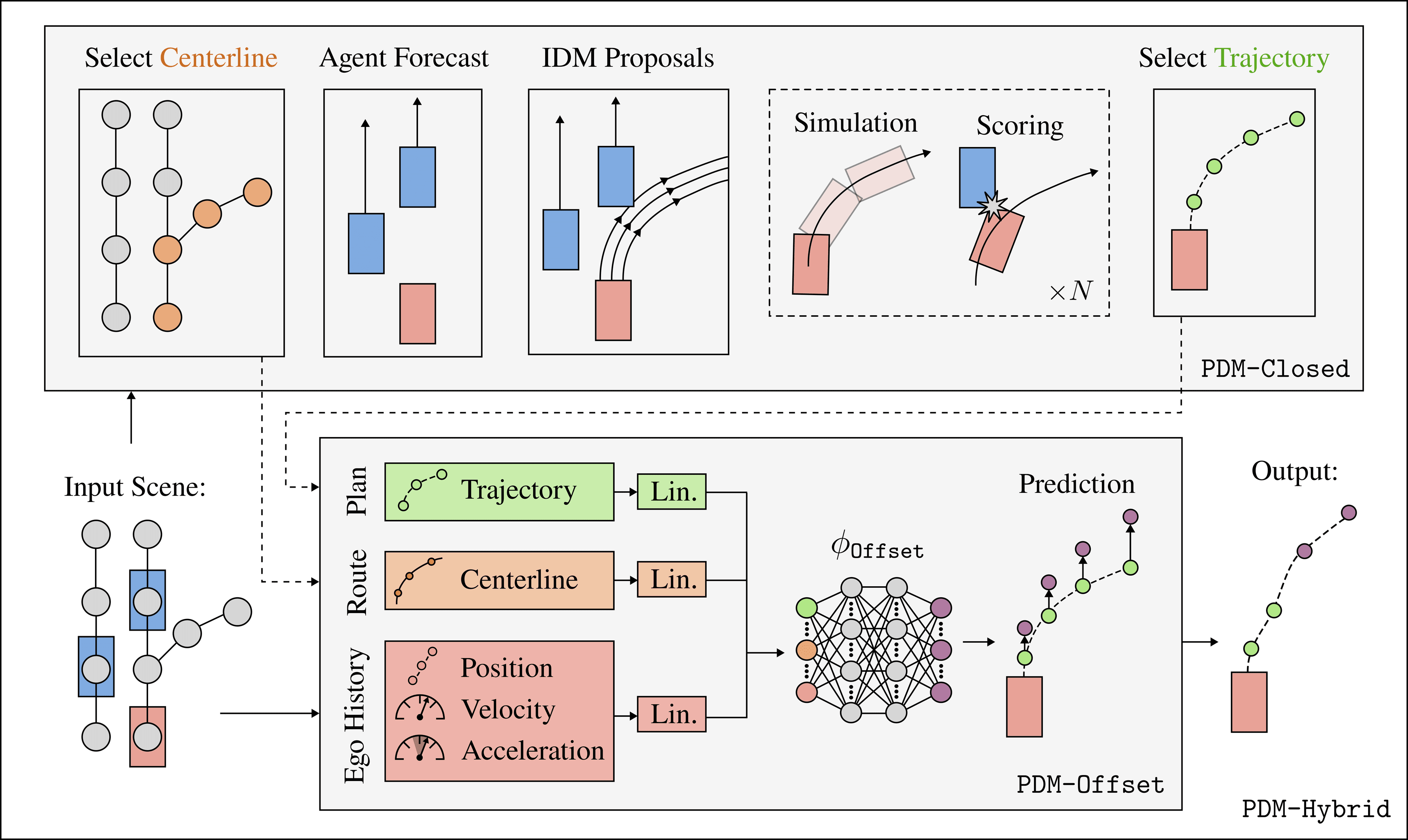
PDM-Closed's mechanism is not sophisticated: generate a small set of proposals using IDM policies at several target speeds and lateral offsets, forward-simulate each proposal with an LQR controller on a bicycle model, score each one against nuPlan's own criteria (collision, drivable area, progress, comfort), and keep the best. In other words, it tries before it commits rather than regressing a trajectory in a single forward pass.
Two takeaways worth carrying:
- Open-loop and closed-loop are different problems, and optimizing one does not automatically improve the other. A learned planner that imitates human drivers beautifully can still fall apart once its own errors start compounding — the classic covariate shift of imitation learning.
- Rule-based is not dead. PDM-Hybrid keeps rules for short-term control and uses the network only for long-horizon forecasting — the only configuration in the table that reaches both CLS 93 and OLS 84.
End-to-end approaches such as UniAD (CVPR 2023 Best Paper) and VAD fold perception, prediction, and planning into one jointly trained network and post impressive nuScenes open-loop numbers. But until there are convincing closed-loop results at nuPlan scale, production stacks — Waymo, Mobileye, comma.ai — keep a verifiable rule layer between the neural network and the actuators.
The end-to-end latency budget
What an L2+ stack actually lives with:
| Stage | Typical budget |
|---|---|
| Sensor capture to usable point cloud/image | 20–50 ms |
| Perception + tracking (Part 3) | 50–100 ms |
| Localization (Part 4) | 10–20 ms |
| Prediction + motion planning | 50–100 ms |
| Control (MPC) | 1–5 ms |
| CAN transmission to actuators | 10–20 ms |
| Total sensor-to-wheel latency | 150–300 ms |
At 100 km/h, 250 ms is 7 meters. That is why every serious planner plans against the predicted state at command execution time, not the state when the sensor fired.
Summary
- Planning splits into four layers because of the compute budget, not architectural taste; each layer has its own horizon and rate.
- The Lanelet2 routing graph turns route finding into graph search, but lane-change cost must be penalized properly or you get kinematically impossible routes.
- The Frenet frame removes curvature from the problem, enabling hundreds of quintic-polynomial candidates filtered by cost and kinematic constraints.
- MPC is the only controller that expresses hard constraints;
Rdand curvature feedforward matter more than newcomers expect. - PDM shows that in closed-loop, a rule set that simulates before it commits still beats learned planners — and a high open-loop score guarantees nothing about that.
In Part 6, the final article of this series, we move from "make it work" to "prove it is safe": ISO 26262 and its ASIL levels, ISO 21448 (SOTIF) for hazards that do not come from component faults, and the Euro NCAP 2026 protocols — the largest revision since 2009.