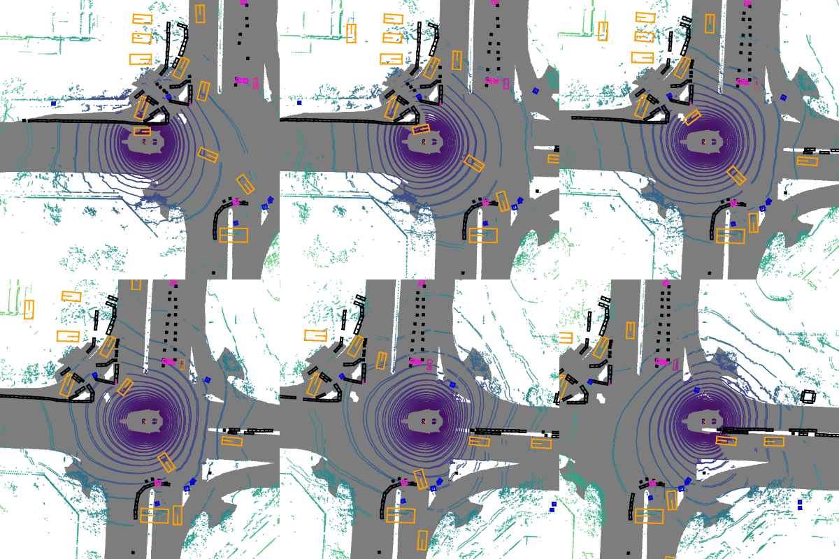
In Part 2 of this series, we built sensor fusion pipelines — early, late, and BEV fusion — that merge camera, LiDAR, and radar streams into a unified feature tensor. A tensor by itself doesn't steer a car, though. The vehicle needs to know what is out there, where things are moving, and which regions of space are safe to enter.
That's exactly where the perception layer comes in. Part 3 walks through three consecutive tasks that convert fused data into actionable scene understanding:
- 3D Object Detection — who is out there? (CenterPoint, DETR3D)
- Occupancy Prediction — which space is occupied? (Occ3D, SurroundOcc)
- Multi-Object Tracking — where are things going? (ByteTrack, OC-SORT)
Series roadmap
- Part 1 — SAE Level 2 vs 2+ vs 3 vs 4: who is responsible for driving, ODD and fallback.
- Part 2 — Sensor fusion: camera, radar and LiDAR building perception that degrades safely.
- Part 3 — Perception: 3D detection, occupancy grids and tracking on nuScenes.
- Part 4 — Localization and HD maps: GNSS/IMU fusion, NDT on LiDAR, map-free approaches.
- Part 5 — Planning and control: from rule-based to MPC and PDM, tracking a real trajectory.
- Part 6 — Validation: ISO 26262, SOTIF and Euro NCAP — proving safety without driving the miles.
Part 1 — 3D Object Detection: CenterPoint and DETR3D
Why 3D and not 2D?
2D camera detection (YOLO, Faster-RCNN) produces pixel bounding boxes — sufficient for recognition but not for control. A self-driving stack needs to know: how far is this object, how tall, how wide, what angle is it facing, and how fast is it moving. 3D object detection returns a 7-DOF box (x, y, z, l, w, h, yaw) plus velocity (vx, vy) — enough for the planner to reason about future collisions.
CenterPoint — detect the center, not the corners
CenterPoint (CVPR 2021, Tianwei Yin et al.) asks a deceptively simple question: instead of predicting four corners of a bounding box — which is highly sensitive to rotation — why not detect the center of mass and regress attributes from there?
Two-stage pipeline:
Stage 1 — Heatmap detection:
The LiDAR point cloud is voxelized, passed through a backbone (VoxelNet or PointPillars) and a pillar/voxel feature network, producing a Bird's Eye View (BEV) feature map. A keypoint head predicts a Gaussian heatmap where peaks correspond to object centers in BEV space. Simultaneously the model regresses: sub-voxel offset (Δx, Δy), height z, dimensions (l, w, h), orientation (sin(yaw), cos(yaw)), and velocity (vx, vy).
Stage 2 — Point-feature refinement: Starting from the predicted center positions, Stage 2 samples additional point features from the surrounding point cloud to refine all attributes. This is what makes CenterPoint particularly strong on small objects and high-speed targets.
nuScenes validation results (MMDetection3D):
| Variant | mAP | NDS | Memory | Note |
|---|---|---|---|---|
| Pillar (0.2) baseline | 48.70 | 59.62 | 4.6 GB | Fastest |
| Voxel (0.1) baseline | 56.11 | 64.61 | 5.2 GB | Balanced |
| Voxel (0.075) baseline | 56.54 | 65.17 | 8.2 GB | Better |
| Voxel (0.075) + DCN + TTA | 60.43 | 67.65 | — | Best |
On the test set: mAP 58.0, NDS 65.5, 11 FPS throughput. Tracking: AMOTA 63.8 — top of the nuScenes leaderboard at publication (2021).
DETR3D — camera-only, no LiDAR required
While CenterPoint relies on LiDAR, DETR3D (CoRL 2022) demonstrates that six surround-view cameras can achieve reasonable 3D detection — critical for cost-sensitive vehicles without LiDAR.
DETR3D extends DETR (Detection Transformer) with a key mechanism: each object query (N learnable vectors) holds a 3D reference point. The detection head projects these 3D points onto each camera's image plane, samples features via bilinear interpolation, and feeds them into transformer decoder cross-attention. There is no explicit 3D representation — all 3D knowledge comes from camera geometry alone.
nuScenes validation set comparison:
| Method | Input | mAP | NDS |
|---|---|---|---|
| DETR3D | Camera × 6 | 0.346 | 0.425 |
| PETR | Camera × 6 | ~0.354 | ~0.433 |
| CenterPoint | LiDAR | 0.561 | 0.646 |
| BEVFusion (cam+LiDAR) | Multimodal | ~0.68 | ~0.72 |
The camera-only vs LiDAR gap remains large (~20 NDS points), but DETR3D established the foundation for all subsequent transformer-based 3D detectors: BEVFormer, PETR, Sparse4D, and beyond.
Code: CenterPoint inference with MMDetection3D
# Install: pip install mmdet3d mmengine
# Download checkpoint from: https://github.com/open-mmlab/mmdetection3d/tree/main/configs/centerpoint

from mmdet3d.apis import init_model, inference_detector

CONFIG = 'configs/centerpoint/centerpoint_voxel01_second_secfpn_8xb4-cyclic-20e_nus-3d.py'
CHECKPOINT = 'checkpoints/centerpoint_voxel01_second_secfpn_8xb4-cyclic-20e_nus-3d-cbgs_20220810_030004-9dfb4232.pth'

# Initialize model on GPU
model = init_model(CONFIG, CHECKPOINT, device='cuda:0')

# nuScenes LiDAR file (.pcd.bin = float32 x,y,z,intensity,timestamp)
PCD_FILE = 'demo/data/nuscenes/n015-2018-07-24-11-22-45+0800__LIDAR_TOP__1532402927647951.pcd.bin'

result, _ = inference_detector(model, PCD_FILE)

# Extract predictions
bboxes = result.pred_instances_3d.bboxes_3d   # tensor (N, 9): x,y,z,l,w,h,yaw,vx,vy
scores = result.pred_instances_3d.scores_3d   # tensor (N,)
labels = result.pred_instances_3d.labels_3d   # tensor (N,) — index into class_names

CLASS_NAMES = [
    'car', 'truck', 'construction_vehicle', 'bus', 'trailer',
    'barrier', 'motorcycle', 'bicycle', 'pedestrian', 'traffic_cone'
]

SCORE_THRESH = 0.3
print(f"Detected {(scores > SCORE_THRESH).sum().item()} objects (threshold={SCORE_THRESH}):\n")

for box, score, label in zip(bboxes, scores, labels):
    if score < SCORE_THRESH:
        continue
    x, y, z, l, w, h, yaw, vx, vy = box.tolist()
    print(
        f"  {CLASS_NAMES[label]:25s} | score={score:.3f} | "
        f"pos=({x:+.1f}, {y:+.1f}, {z:+.1f}) m | "
        f"size=({l:.1f}×{w:.1f}×{h:.1f}) | "
        f"yaw={yaw:.2f} rad | "
        f"vel=({vx:+.1f}, {vy:+.1f}) m/s"
    )
Sample output (nuScenes scene):
Detected 18 objects (threshold=0.3):

  car                       | score=0.871 | pos=(+8.4, +2.1, -0.8) m | size=(4.5×2.0×1.6) | yaw=0.02 rad | vel=(+0.1, +0.0) m/s
  pedestrian                | score=0.743 | pos=(-3.2, +8.5, -0.3) m | size=(0.7×0.7×1.8) | yaw=-1.57 rad | vel=(-0.5, +1.2) m/s
  bicycle                   | score=0.412 | pos=(+15.3, -1.4, -0.5) m | size=(1.8×0.6×1.3) | yaw=0.05 rad | vel=(+2.1, +0.0) m/s
  ...
From a single LiDAR frame, we have full 3D information for every detected object — centimeter-level precision, plus velocity for planning.
Part 2 — Occupancy Prediction: Occ3D and SurroundOcc
Why bounding boxes aren't enough
Imagine a pile of construction debris blocking a lane. What does a bounding box detector do? If "debris" is not in the class vocabulary — the model ignores it. If it is, a bounding box crudely wraps an irregular shape in a rectangular prism that conveys nothing about actual geometry.
This is the long-tail problem of bounding box detection:
- Training datasets only label predefined classes (car, truck, pedestrian...)
- Unusual objects (overturned vehicles, fallen cargo, construction barriers) are unlabeled
- The model learns nothing about them → dangerous blind spots
Occupancy prediction reframes the question entirely: instead of "is there an object here?", it asks "is this voxel occupied?" — and if so, what type of material is it?
Occ3D — the standard benchmark (NeurIPS 2023)
Occ3D introduces a large-scale benchmark derived from nuScenes, dividing the surrounding 3D space into a dense voxel grid:
- Prediction range: X ∈ [-40m, 40m], Y ∈ [-40m, 40m], Z ∈ [-1m, 5.4m]
- Voxel resolution: 0.4m × 0.4m × 0.4m
- Grid size: 200 × 200 × 16 = 640,000 voxels per frame
- Classes: 17 semantic classes + 1 empty
- Primary metric: mIoU (mean Intersection over Union) across 18 classes
Every voxel carries a semantic label — from car (class 1) to terrain (class 11) to empty (class 0). If a voxel contains LiDAR returns from a car, it's labeled car. If it contains concrete sidewalk, it's sidewalk. If nothing is present, it's empty.
Crucially: unknown objects that can't be classified still get labeled as other_flat_surface or other_object — they are never silently ignored.
SurroundOcc — camera-only occupancy (ICCV 2023)
SurroundOcc (Wei et al., ICCV 2023) solves the same task using only cameras, without requiring direct LiDAR annotation at inference time.
Architecture:
- Multi-scale image encoding: Each camera image (6 total) goes through a ResNet-101 backbone, producing multi-scale feature pyramids.
- Spatial cross-attention (BEV lift): Learnable 3D queries — one per voxel — attend to the relevant image features via projection (similar to BEVFormer, but volumetric instead of planar).
- Temporal aggregation: Features from the current and previous frames are fused to improve depth estimation.
- Occupancy head: A 3D CNN decoder produces dense voxel-level semantic predictions.
Dataset comparison:
| Benchmark | X/Y range | Z range | Voxel size | Grid | Classes |
|---|---|---|---|---|---|
| Occ3D-nuScenes | ±40m | -1m → 5.4m | 0.4m³ | 200×200×16 | 17+1 |
| SurroundOcc | ±50m | -5m → 3m | 0.5m³ | 200×200×16 | 16+1 |
SurroundOcc extends the prediction horizon (±50m vs ±40m) and increases Z coverage (from -5m — useful for underpasses and ramps).

Occupancy vs Detection: when to use which?
| Criterion | Bounding Box | Occupancy |
|---|---|---|
| Compute cost | Low | High (640k voxels/frame) |
| Long-tail handling | Poor | Good |
| Geometry accuracy | Medium | High |
| Planning integration | Simple | More complex |
| Annotation cost | Low (box labels) | High (dense LiDAR scan) |
In production systems: Tesla FSD replaced bounding boxes entirely with occupancy networks in FSD v11 (2023). Waymo uses both — bounding boxes for tracking, occupancy for free-space estimation.
Part 3 — Multi-Object Tracking: ByteTrack and OC-SORT
If detection tells us "at frame T, there is a car at position (8.4m, 2.1m)", tracking must answer: "Which car is this? And at frame T+1, where is it?" — maintaining consistent identity over time.
Key metrics on nuScenes
The nuScenes Tracking Benchmark uses five primary metrics:
| Metric | Meaning | Better when |
|---|---|---|
| AMOTA | Average Multi-Object Tracking Accuracy | Higher |
| AMOTP | Average Multi-Object Tracking Precision | Lower |
| MOTA | Tracking accuracy at fixed recall | Higher |
| IDS | Identity Switches | Lower |
| FRAG | Track Fragmentation | Lower |
AMOTA is the primary metric: it averages MOTA over multiple recall thresholds (0.1 to 1.0, step 0.1) — making it robust against models that detect few objects with high precision vs. models that detect many objects with some noise.
AMOTP measures average localization error of true positive tracks — in meters. Lower is better.
IDS (ID Switches) is arguably the most operationally significant: every identity switch means the prediction module loses that object's motion history and must restart, potentially causing abrupt braking or unstable behavior.
ByteTrack — don't waste any detection
ByteTrack (ECCV 2022) starts from a simple observation: most trackers only associate high-confidence detections (score > 0.5) with existing tracks, discarding low-confidence ones. But low-confidence detections often represent real objects that are occluded, far away, or at difficult angles.
Two-stage association:
- Stage 1: Hungarian assignment between all existing tracks and high-conf detections (score > τ_high ≈ 0.5) using BEV IoU distance.
- Stage 2: Unmatched tracks from Stage 1 are associated with low-conf detections (τ_low < score < τ_high). If IoU is sufficient, the track is kept alive; otherwise it enters a "lost" state.
Results: ByteTrackV2 achieves 54.2 AMOTA and 696 IDS on nuScenes validation (camera-based), outperforming the second-ranked method by 3.1 AMOTA.
OC-SORT — fixing drift during occlusion
OC-SORT (Observation-Centric SORT, CVPR 2023) addresses a fundamental failure mode of standard Kalman filters: when an object is occluded for several frames, Kalman updates occur using predicted state only (no real observation) — causing drift (accumulated estimation error). When the object reappears, the track has drifted to the wrong position → identity switch.
OC-SORT addresses this with two techniques:
- Observation-Centric Re-Update: When a track re-emerges after occlusion, OC-SORT recomputes the trajectory based on direct observations before and after the occlusion gap — removing the influence of phantom state updates.
- Observation-Centric Momentum: The velocity term in the Kalman filter is estimated from the two most recent actual observations, not from the state chain — preventing error accumulation.
When to use each tracker:
| Scenario | Recommendation |
|---|---|
| Straight highway, minimal occlusion | ByteTrack (simpler, faster) |
| Urban driving, frequent occlusion | OC-SORT (fewer ID switches) |
| Strong camera motion, nonlinear trajectories | OC-SORT (stable velocity model) |
| Hard real-time requirement | ByteTrack (lower compute) |
nuScenes tracking benchmark comparison:
| Method | Detector | AMOTA ↑ | AMOTP ↓ | IDS ↓ |
|---|---|---|---|---|
| CenterPoint (LiDAR) | CenterPoint | 63.8 | 0.555 | — |
| ByteTrackV2 (camera) | — | 54.2 | — | 696 |
| S2-Track (SOTA 2024) | — | 66.3 | — | — |
CenterPoint's built-in tracker remains highly competitive thanks to LiDAR data quality. Camera-based trackers (ByteTrackV2) trail by ~10 AMOTA — the gap comes from depth estimation uncertainty propagating into the tracker state.
The complete perception pipeline
LiDAR + Camera + Radar
         │
    [Sensor Fusion]       ← (BEVFusion — Part 2)
         │
    [3D Detection]        ← CenterPoint / DETR3D
         │                → boxes: (x,y,z,l,w,h,yaw,vx,vy,class,score)
    [Occupancy]           ← Occ3D / SurroundOcc
         │                → dense voxel grid (640k labels/frame)
    [MOT Tracker]         ← ByteTrack / OC-SORT
         │                → tracks: {id, state_history, velocity_estimate}
    [Trajectory Pred.]    ← Social-LSTM, Trajectron++
         │                → future trajectories (T+1s to T+5s)
    [Planning]            ← (Part 5)
Tracking is the bridge between perception (knowing where things are now) and prediction (knowing where they'll be next). A single ID switch doesn't just hurt a benchmark number — it means the prediction module loses an object's motion context and restarts cold.
Summary
The three perception layers in this post build incrementally:
- 3D Detection (CenterPoint/DETR3D) identifies who is present and their 3D shape.
- Occupancy Prediction (Occ3D/SurroundOcc) fills in the gaps — every occupied voxel is known, whether it's a familiar class or an out-of-vocabulary long-tail obstacle.
- Tracking (ByteTrack/OC-SORT) assigns persistent identities so the planner knows "this specific vehicle has been accelerating for the past 2 seconds".
Next up: Part 4 — Localization and HD Maps tackles the complementary question: where is the vehicle itself within the map? — at centimeter precision, not GPS-level 3 meters.