In Part 3 of this series, we explored how the perception system identifies surrounding objects — other vehicles, pedestrians, traffic signs — through 3D object detection and occupancy grids. But knowing what is around you is only half the problem. To plan a safe trajectory, the vehicle needs to know precisely where it is on the road.
This is the localization problem — and it is significantly harder than it first appears.
Consider a practical example: smartphone GPS is typically accurate to 3–10 m. For a human driver, that error is perfectly acceptable — you can see the lane markings and self-correct. But for an autonomous vehicle, a 3 m error is enough to cause a lane departure or miss a critical braking point. ADAS systems need accuracy below 10 cm, ideally 2–5 cm at the lateral (cross-lane) axis.
This article covers three layers of modern autonomous vehicle localization:
- GNSS/IMU fusion — and why RTK-GNSS alone is insufficient
- LiDAR-based localization — NDT vs ICP vs Monte Carlo, with real benchmark numbers
- HD Maps — Lanelet2 vs OpenDRIVE, and map-free approaches with MapTR and StreamMapNet
Series roadmap
- Part 1 — SAE Level 2 vs 2+ vs 3 vs 4: who is responsible for driving, ODD and fallback.
- Part 2 — Sensor fusion: camera, radar and LiDAR building perception that degrades safely.
- Part 3 — Perception: 3D detection, occupancy grids and tracking on nuScenes.
- Part 4 — Localization and HD maps: GNSS/IMU fusion, NDT on LiDAR, map-free approaches.
- Part 5 — Planning and control: from rule-based to MPC and PDM, tracking a real trajectory.
- Part 6 — Validation: ISO 26262, SOTIF and Euro NCAP — proving safety without driving the miles.
Layer 1: GNSS/IMU Fusion — Foundation and Limitations
RTK-GNSS: Impressive but Insufficient
RTK-GNSS (Real-Time Kinematic Global Navigation Satellite System) is an advanced form of GPS. Rather than using a single standalone receiver, RTK combines measurements from the vehicle's receiver with a fixed nearby base station, using carrier phase measurements instead of just pseudorange codes. Theoretical accuracy: 2–3 cm under ideal conditions.
The problem is that ideal conditions rarely exist on real roads.
Urban canyons are the primary enemy. When a vehicle passes through a city center with tall buildings, satellite signals are blocked and reflected multiple times before reaching the receiver — a phenomenon called multipath. Signals arriving via indirect paths (NLOS — Non-Line-of-Sight) are time-shifted, causing the receiver to calculate incorrect positions. In severe urban canyons, RTK-GNSS errors can exceed 10 m — completely useless for autonomous driving.
Tunnels are even worse: no signal at all. The vehicle loses all satellite reference for the entire duration of the tunnel, with no natural recovery mechanism.
IMU: The Bridge with a Time Limit
An Inertial Measurement Unit (IMU) measures acceleration and angular velocity via accelerometers and gyroscopes. By integrating twice (acceleration → velocity → position), an IMU can estimate relative position from a known starting point — requiring no external signals whatsoever.
But IMUs have a fatal flaw: drift. Small measurement errors accumulate over time. For consumer-grade IMUs, drift can reach 0.5–1% of traveled distance. This means after 100 m, the IMU estimate has drifted 50–100 cm from reality. After 1 km in a tunnel, the error can reach 5–10 m.
IMU errors are typically classified into two categories:
- Deterministic errors: bias and scale factor — measurable and correctable at calibration time
- Stochastic errors: random noise, bias instability, random walk — require probabilistic modeling, cannot be fully eliminated
Extended Kalman Filter: Combining Both
The standard solution is GNSS/IMU fusion using an Extended Kalman Filter (EKF). The EKF maintains an estimated state (position, velocity, orientation) along with a covariance matrix representing confidence.
Predict step (runs at IMU frequency, typically 100–400 Hz):
x̂_k = f(x̂_{k-1}, u_k)    # Integrate IMU measurements
P_k = F·P_{k-1}·Fᵀ + Q    # Covariance prediction (Q = process noise)
Update step (runs when GNSS is available, typically 10 Hz):
K = P_k·Hᵀ·(H·P_k·Hᵀ + R)⁻¹   # Kalman gain
x̂_k = x̂_k + K·(z_k - H·x̂_k)  # State update with GNSS measurement z_k
P_k = (I - K·H)·P_k              # Covariance update
When GNSS is lost (tunnel, urban canyon), the system continues predicting via IMU while covariance grows (confidence decreases). When GNSS recovers, the update step pulls the estimate back toward reality and resets covariance.
Result: GNSS/IMU fusion typically achieves 10–30 cm accuracy in good conditions. Still insufficient for lane-level navigation — which is why we need a third layer.
Layer 2: LiDAR-Based Localization — Sub-5 cm Accuracy
The core idea: if we have a point cloud map of the environment (collected in advance and georeferenced), we can match the current LiDAR scan against that map to localize with far greater precision than GNSS alone.
This process — scan matching or map-based localization — is the dominant technique in production autonomous driving systems.
NDT: Normal Distribution Transform
NDT (Normal Distribution Transform) is the scan matching algorithm used by Autoware and many production autonomous driving systems. The approach:
- Divide the 3D space into voxels (typically 1–2 m per side)
- For each map voxel, compute a Gaussian distribution over the points inside (mean vector and covariance matrix)
- For a new LiDAR scan, find the rigid transformation (R, t) that maximizes the probability of scan points falling within the correct map Gaussian distributions
Optimization objective (negative log-likelihood):
T* = argmin_T -Σᵢ exp(-½·(x̃ᵢ - μᵢ)ᵀ·Σᵢ⁻¹·(x̃ᵢ - μᵢ))
Where x̃ᵢ = R·xᵢ + t is the transformed scan point, and μᵢ, Σᵢ are the mean and covariance of the corresponding map voxel.
Why is NDT better than raw point-to-point comparison? The Gaussian representation smooths discrete points and handles environmental changes more robustly (different parked cars each day, seasonal foliage changes, varying lighting). The map does not need to match reality perfectly — the Gaussian distribution has enough flexibility to absorb small differences.
ICP: Iterative Closest Point
ICP is a more intuitive approach: find the transformation that minimizes the average distance between each scan point and its nearest neighbor in the map.
T* = argmin_T Σᵢ ||T·xᵢ - yᵢ||²
Where yᵢ is the nearest map point to T·xᵢ. The algorithm alternates between finding correspondences (nearest neighbor search) and optimizing the transform (closed-form solution).
ICP is simple and achieves high accuracy given a good initial estimate, but is sensitive to outliers (dynamic objects like moving vehicles and pedestrians) and prone to local minima in environments with repetitive structure (long corridors, smooth walls).
Monte Carlo Localization
MCL (Monte Carlo Localization), also known as Particle Filter, takes a completely different approach: instead of optimizing a single pose, MCL maintains a set of particles (N = 1,000–10,000 hypotheses about the vehicle's position).
# Each particle = (x, y, theta, weight)
particles = [(x_i, y_i, theta_i, w_i) for i in range(N)]

# Motion update: propagate particles with noise from motion model
particles = [motion_model(p, delta_x, delta_y, delta_theta) for p in particles]

# Sensor update: weight particles by LiDAR scan likelihood
particles = [(p[0], p[1], p[2], sensor_model(scan, map, p)) for p in particles]

# Resample proportional to weight
particles = resample(particles)
MCL's unique strength is handling the kidnapped robot problem — when the vehicle is suddenly displaced (e.g., transported by a flatbed), MCL can recover by distributing new particles globally and converging on the correct location.
Algorithm Comparison
| Algorithm | Strengths | Weaknesses | Typical Lateral RMSE |
|---|---|---|---|
| NDT | Robust to environmental change, GPU-parallelizable, efficient | Sensitive to voxel size, needs good GNSS initial guess | 1.6–4 cm |
| ICP | Simple, high accuracy with good initialization | Sensitive to outliers, local minima in repetitive environments | 2–6 cm |
| MCL | Multi-hypothesis, recovery from kidnapping, principled probabilistic | High RAM/CPU for large particle counts, lower accuracy than NDT | 5–15 cm |
Real benchmarks: IEEE ITSC 2019 research (Pang et al.) measured NDT achieving MAE of 4.06 cm at low speed (5–10 mph) and 5.42 cm at moderate speed (15–20 mph). On highway datasets with high-quality maps, Autoware NDT achieves lateral RMSE of 1.6 cm, maximum error 7.6 cm (from Robust Localization for Highway Scenes, arXiv 2604.22040).
Running NDT Localization with Autoware.Universe
Autoware.Universe is the most widely-used open-source autonomous driving stack in research and industry. Here is how to run NDT localization with sample data:
Step 1: Setup (Docker recommended)
git clone https://github.com/autowarefoundation/autoware.git
cd autoware
./setup-dev-env.sh docker
source install/setup.bash
Step 2: Launch with NDT as pose estimator
ros2 launch autoware_launch autoware.launch.xml \
  map_path:=/path/to/your/map \
  vehicle_model:=sample_vehicle \
  sensor_model:=sample_sensor_kit \
  pose_source:=ndt \
  twist_source:=gyro_odometer
Step 3: Measure lateral RMSE
#!/usr/bin/env python3
"""
Measure lateral RMSE for NDT localization.
Requires: ground truth pose from RTK or simulation (AWSIM).
"""

import rclpy
from rclpy.node import Node
from nav_msgs.msg import Odometry
import numpy as np
from collections import deque

class LocalizationEvaluator(Node):
    def __init__(self):
        super().__init__('localization_evaluator')

        self.est_sub = self.create_subscription(
            Odometry,
            '/localization/kinematic_state',
            self.est_callback, 10
        )
        self.gt_sub = self.create_subscription(
            Odometry,
            '/ground_truth/odom',  # From AWSIM or RTK reference
            self.gt_callback, 10
        )

        self.est_poses = deque(maxlen=1000)
        self.gt_poses = deque(maxlen=1000)
        self.lateral_errors = []

    def est_callback(self, msg):
        t = msg.header.stamp.sec + msg.header.stamp.nanosec * 1e-9
        x = msg.pose.pose.position.x
        y = msg.pose.pose.position.y
        self.est_poses.append((t, x, y))
        self._compute_error()

    def gt_callback(self, msg):
        t = msg.header.stamp.sec + msg.header.stamp.nanosec * 1e-9
        x = msg.pose.pose.position.x
        y = msg.pose.pose.position.y
        self.gt_poses.append((t, x, y))

    def _compute_error(self):
        if not self.est_poses or not self.gt_poses:
            return

        est_t, est_x, est_y = self.est_poses[-1]
        gt_times = np.array([p[0] for p in self.gt_poses])
        closest_idx = np.argmin(np.abs(gt_times - est_t))

        if abs(gt_times[closest_idx] - est_t) > 0.1:
            return  # Skip if time gap > 100 ms

        _, gt_x, gt_y = self.gt_poses[closest_idx]
        error = np.sqrt((est_x - gt_x)**2 + (est_y - gt_y)**2)
        self.lateral_errors.append(error)

    def print_stats(self):
        if self.lateral_errors:
            errors = np.array(self.lateral_errors)
            self.get_logger().info(
                f"Lateral RMSE: {np.sqrt(np.mean(errors**2))*100:.1f} cm | "
                f"MAE: {np.mean(errors)*100:.1f} cm | "
                f"Max: {np.max(errors)*100:.1f} cm | "
                f"N: {len(errors)}"
            )

def main():
    rclpy.init()
    evaluator = LocalizationEvaluator()
    try:
        rclpy.spin(evaluator)
    except KeyboardInterrupt:
        evaluator.print_stats()
    finally:
        evaluator.destroy_node()
        rclpy.shutdown()

if __name__ == '__main__':
    main()
Typical results on AWSIM (Autoware virtual environment):
Lateral RMSE: 1.8 cm | MAE: 1.4 cm | Max: 4.2 cm | N: 3421
This is the accuracy level that Waymo and Mobileye require for lane-keeping and trajectory planning. RTK-GNSS alone cannot reliably achieve this in real urban environments.
Layer 3: HD Maps — The Vehicle's Semantic Knowledge Base
The point cloud map used in Layer 2 tells the vehicle exactly where it is. But the vehicle also needs to know the meaning of the environment: which lanes are legal to drive in, what is the speed limit here, which traffic light governs this intersection?
This is the role of the HD Map — and it is fundamentally different from navigation maps like Google Maps or Apple Maps.
| Criterion | Navigation Map (Google Maps) | HD Map (for ADAS) |
|---|---|---|
| Accuracy | 3–10 m | 5–20 cm |
| Smallest unit | Road | Individual lane |
| Update frequency | Weekly/monthly | Realtime or daily |
| Content | Turn-by-turn, POI | Lane markings, signs, curvature, speed limits |
OpenDRIVE: The Simulation Standard
OpenDRIVE is an XML format developed by ASAM (Association for Standardization of Automation and Measuring Systems). It describes road networks through three layers:
- Reference line: the road's central axis, described by geometric primitives (straight lines, circular arcs, Euler spirals/clothoids)
- Lane sections: lanes derived from the reference line, with offset and width as functions of road distance (s-coordinate)
- Objects and signals: road signs, traffic lights, obstacles attached to the road via Frenet coordinates (s, t)
OpenDRIVE excels at simulation: CARLA, SUMO, and LGSVL all use it natively. However, it is complex to build and maintain for production fleets.
Lanelet2: The Operational Standard
Lanelet2 was developed by FZI Research Center (Germany) and is the defacto standard for Autoware.Universe and many production systems. It organizes maps using 6 primitives in a clear hierarchy:
Point → LineString → Polygon
                  ↘
                   Lanelet → Area
                            ↘
                             RegulatoryElement
- Point: 3D coordinates (lat/lon/ele or XYZ) with optional attributes
- LineString: ordered sequence of points — represents lane markings, curb edges, lane boundaries
- Polygon: closed region (parking lots, no-go zones)
- Lanelet: a directed lane unit — defined by a left LineString and a right LineString
- Area: undirected region (complex intersections, roundabouts)
- RegulatoryElement: traffic rules applied to lanelets/areas (speed limits, traffic lights, yield signs)
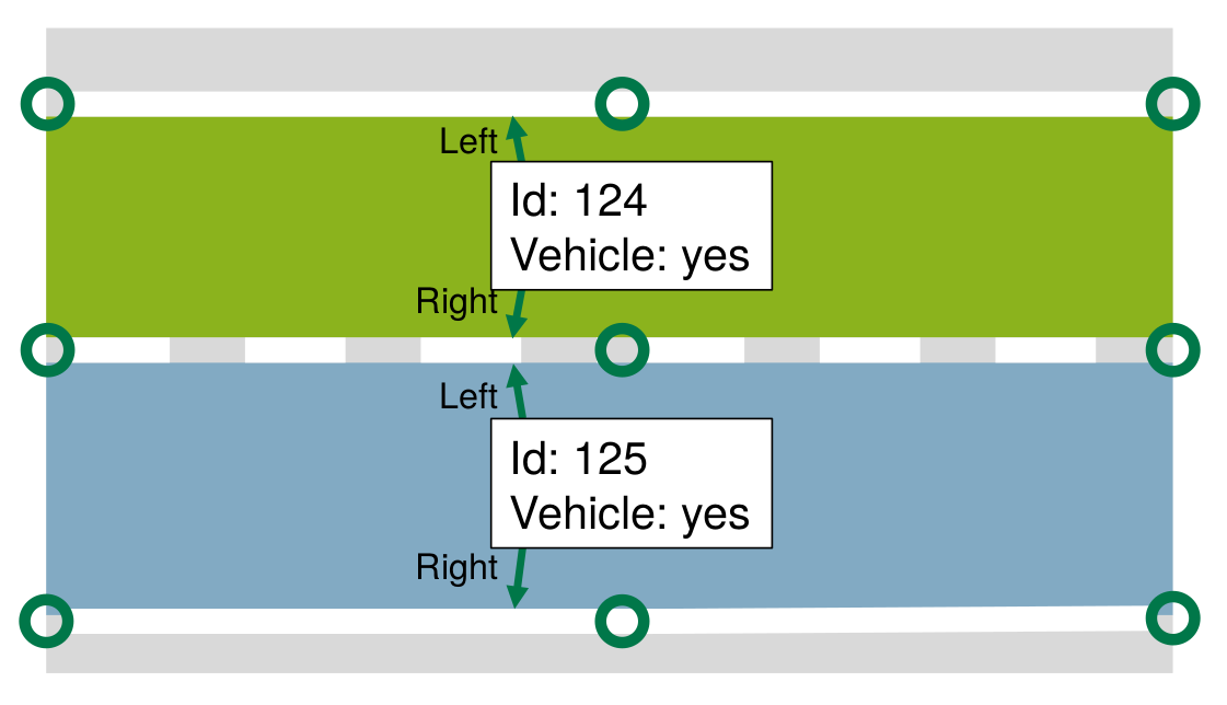
A single Lanelet: left boundary (blue), right boundary (red), and the automatically computed centerline (middle). Source: FZI Research Center / Lanelet2 repo
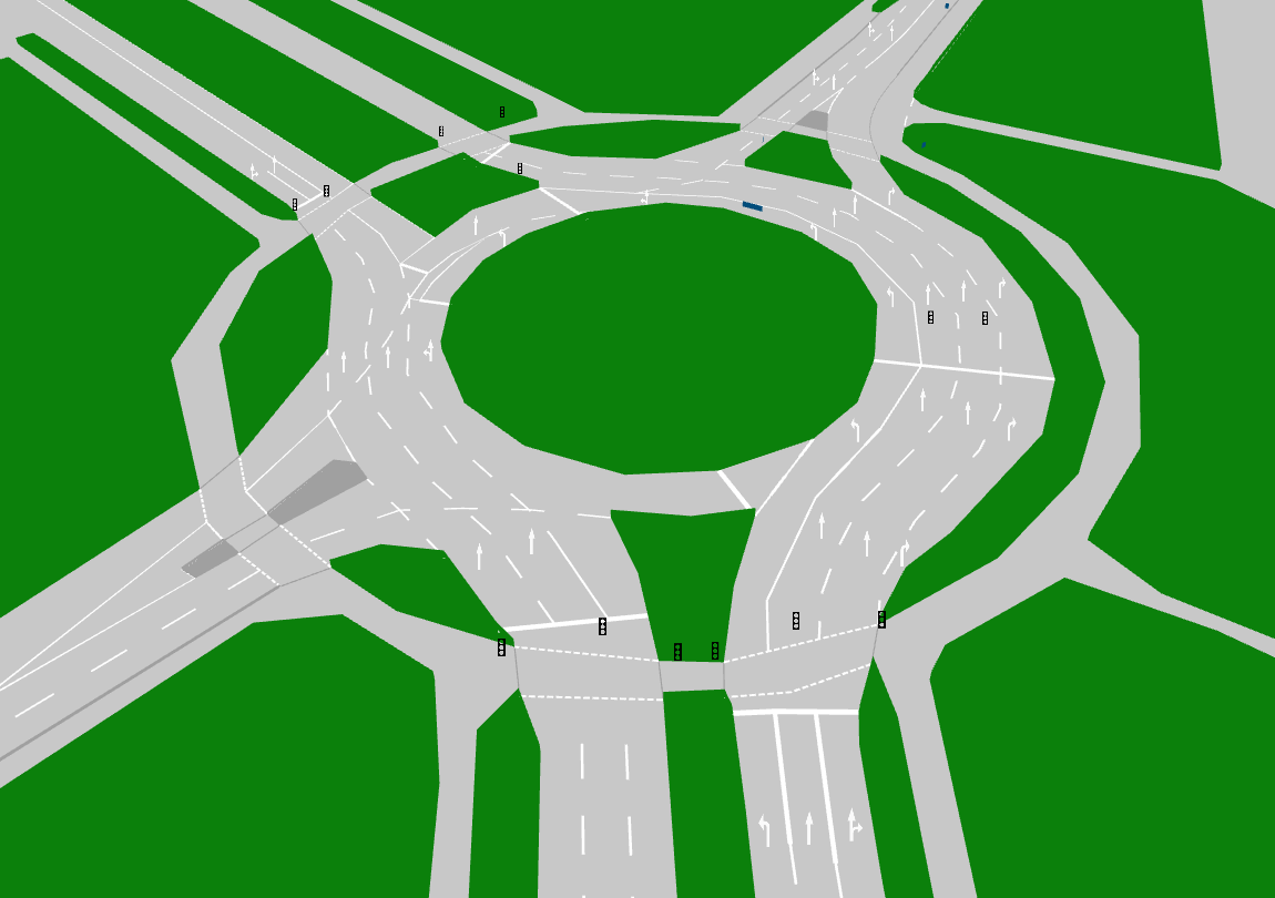
A Lanelet2 map of a complex road segment: directed lanelets (different colors per direction), intersection areas, and regulatory elements (traffic lights, stop lines). Source: FZI Research Center / Lanelet2 repo
A practical example of creating a Lanelet using the Lanelet2 Python API:
import lanelet2
from lanelet2.core import Point3d, LineString3d, Lanelet

# Create boundary points
left_pts = [
    Point3d(1, 100.0, 0.0, 0.0),   # (id, x, y, z)
    Point3d(2, 200.0, 0.0, 0.0),
]
right_pts = [
    Point3d(3, 100.0, -3.5, 0.0),  # 3.5 m standard lane width
    Point3d(4, 200.0, -3.5, 0.0),
]

# Create LineStrings — "dashed" = lane change permitted
left_ls = LineString3d(5, left_pts, {"type": "line_thin", "subtype": "dashed"})
# "solid" = no lane change allowed
right_ls = LineString3d(6, right_pts, {"type": "line_thin", "subtype": "solid"})

# Create Lanelet with semantic attributes
ll = Lanelet(7, left_ls, right_ls)
ll.attributes["subtype"] = "road"
ll.attributes["speed_limit"] = "60"    # km/h
ll.attributes["location"] = "urban"

# Centerline is computed automatically from left + right boundary
centerline = ll.centerline
print(f"Lane length: {lanelet2.geometry.length(centerline):.1f} m")
# Output: Lane length: 100.0 m
OpenDRIVE vs Lanelet2 Comparison
| Criterion | OpenDRIVE | Lanelet2 |
|---|---|---|
| Format | XML (ASAM spec) | OSM-based XML |
| Primary use | Simulation (CARLA, SUMO) | Production driving (Autoware, Apollo) |
| Road representation | Reference line + derived lanes | Direct Point/LineString geometry |
| Topology graph | Less explicit | Explicit routing graph |
| Traffic rules | Embedded in lane definitions | Separate RegulatoryElement objects |
| Tooling | Commercial (RoadRunner) + open spec | Fully open C++ library + Python bindings |
| Strength | Complex geometry (clothoid curves) | Rich semantics, easy topology queries |
Map-Free Approaches: MapTR and StreamMapNet
High-quality HD maps are extremely expensive to build and maintain: they require dedicated mapping vehicles, manual annotation labor, and continuous update processes as roads change, construction occurs, or signs are replaced. Building and maintaining HD map coverage for a major city can cost tens of millions of dollars.
Recent research focuses on online map construction — the vehicle builds the map in real-time directly from sensor input, without relying on a pre-built HD map.
MapTR: Transformer-Based Vectorized Map from Cameras
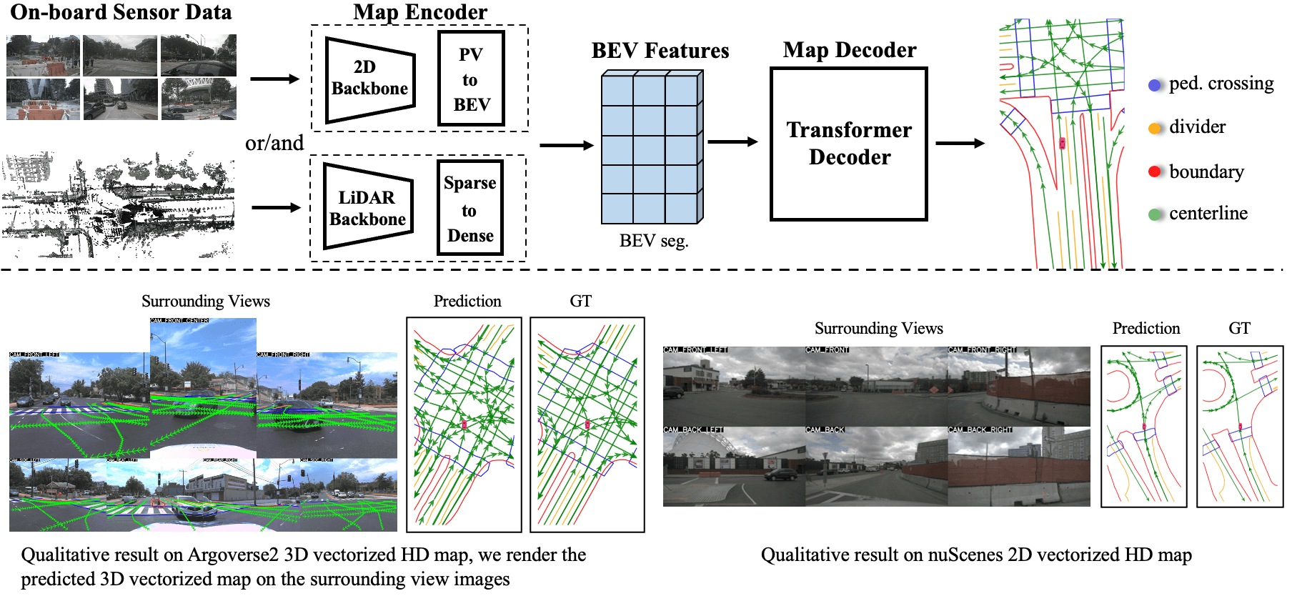
MapTR (ICLR 2023, MapTRv2 published in IJCV 2024) is an end-to-end framework using Vision Transformers to construct vectorized HD maps from surround-view cameras alone — no LiDAR required.
The core innovation is permutation-equivalent modeling: a map element (lane divider, pedestrian crossing, road boundary) is represented as a polyline with a cyclically ordered point set — no fixed start or end point. This resolves the labeling ambiguity in supervised learning where a curve can be annotated starting from either endpoint.
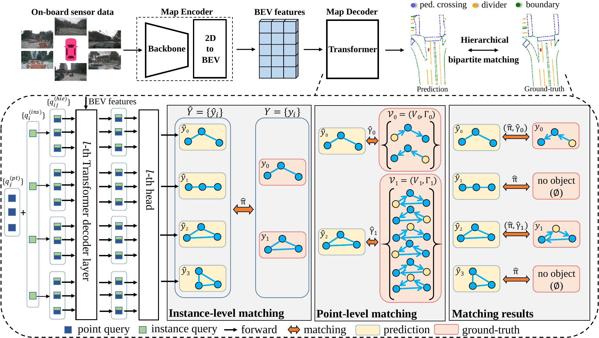
MapTR pipeline: image backbone → BEV feature encoding → Transformer map decoder → vectorized output (lane dividers, pedestrian crossings, road boundaries). Source: hustvl/MapTR repo
MapTR architecture:
- Image backbone + FPN: extract features from 6 cameras (front, front-left, front-right, rear, rear-left, rear-right)
- BEV Encoder: lift image features to Bird's Eye View space
- Map Decoder: Transformer decoder with learnable map element queries
- Permutation-equivalent loss: compare predicted polylines to ground truth over all cyclic permutations, take minimum
Benchmark on nuScenes validation (camera-only, IoU threshold 0.5):
| Method | mAP (divider) | mAP (ped crossing) | mAP (boundary) | Overall mAP | FPS |
|---|---|---|---|---|---|
| HDMapNet | 40.6 | 18.7 | 39.5 | 32.9 | 3.0 |
| VectorMapNet | 50.3 | 36.1 | 42.7 | 43.0 | 4.9 |
| MapTR | 58.9 | 60.5 | 59.7 | 59.7 | 11.1 |
| MapTRv2 | 73.4 | 69.6 | 73.7 | 72.2 | 9.0 |
MapTRv2 improves further by adding an auxiliary dense segmentation head and instance-level augmentation, achieving mAP 72.2 — nearly double HDMapNet's score from just two years prior.
StreamMapNet: Temporal Modeling for Map Stability
StreamMapNet (WACV 2024) addresses MapTR's key weakness: processing each frame independently causes map jitter between consecutive frames — a lane divider might be detected in one frame and missed in the next. This instability is problematic for downstream planning.
StreamMapNet adds streaming temporal modeling: it maintains a BEV feature memory from previous frames, using multi-point cross-attention so the decoder can reference historical information. Results: more stable map predictions, increased map range (from 60 m to 100 m), and higher overall accuracy.
Frame t-3 → BEV feat ──┐
Frame t-2 → BEV feat ──┼──→ Temporal Memory → Map Decoder → Stable Map
Frame t-1 → BEV feat ──┘         ↑
Frame t   → BEV feat ─────────────┘ (current query + temporal context)
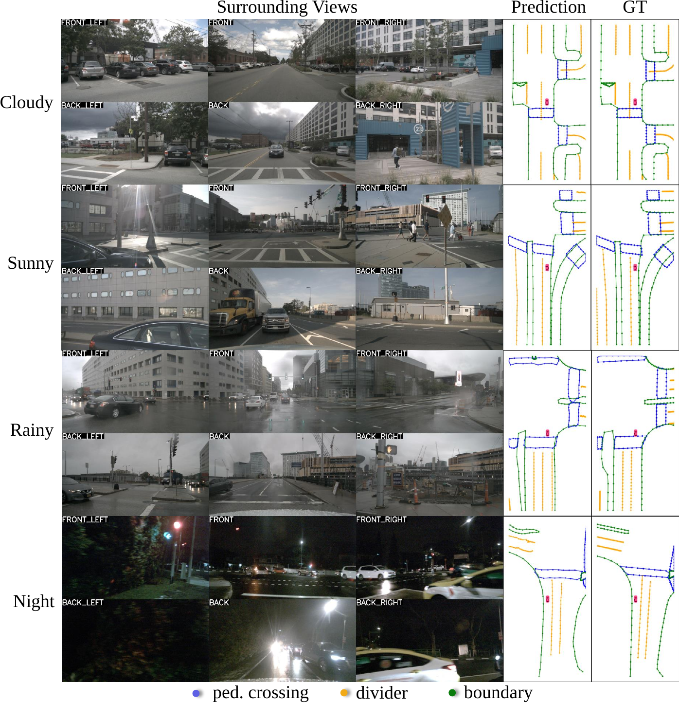
MapTR results on nuScenes: lane dividers, pedestrian crossings, and road boundaries accurately detected from camera-only input. Source: hustvl/MapTR repo
Trade-off: Pre-built HD Map vs Online Map
| Criterion | Pre-built HD Map | Online Map (MapTR/StreamMapNet) |
|---|---|---|
| Accuracy | High (~cm, survey-verified) | Lower (~10–30 cm) |
| Coverage | Only mapped regions | Everywhere (including new roads) |
| Build cost | Very high (fleet mapping + annotation) | Low (self-updating from production data) |
| Robustness to change | Poor (outdated map is dangerous) | Good (always reflects current state) |
| Runtime compute | Near-zero (lookup) | Significant (Transformer inference) |
| Best suited for | Robotaxi within fixed ODD | Consumer ADAS, geofence expansion |
The 2025–2026 trend is a hybrid approach: pre-built HD map serves as the primary source when available (high-density urban cores), with automatic fallback to online map construction for unmapped regions. Multiple major autonomous driving companies are pursuing this direction under various names.
The Complete Localization Pipeline
Combining all three layers, a production-grade localization pipeline in Autoware.Universe looks like this:
GNSS Receiver ──→ gnss_poser ──→ EKF Localizer ──────────→ ┐
                                       ↑                     │
LiDAR Scan ──→ ndt_scan_matcher ───────┘                     ├──→ /localization/kinematic_state
IMU ──────────────────────────────────→ EKF Input            │    (pose + covariance + velocity)
                                                             │
Point Cloud Map ──→ map_loader ──────────────────────────────┘

Lanelet2 Map ──→ map_loader ──→ route_handler ──→ Behavior Planner
                                    ↓
                           Traffic rules, Lane topology
                           Speed limits, Traffic light positions
Each component publishes and subscribes via standard Autoware ROS 2 topics, making the system modular. Individual components can be swapped (replacing NDT with ICP, or GNSS with V2X positioning) without redesigning the full stack.
Summary
Localization is the precise spatial anchor that makes everything else in autonomous driving possible:
- GNSS/IMU fusion provides a 10–30 cm baseline, but is defeated by urban canyons and tunnels
- NDT LiDAR localization narrows this to 1.6–5 cm — the core technology in production autonomous vehicles today
- Lanelet2 HD Maps provide the semantic layer — lanes, traffic rules — that point cloud maps cannot offer
- MapTR/StreamMapNet enable map-free approaches, reducing infrastructure cost but still trailing pre-built maps in accuracy
In Part 5, we will use the precise pose from localization and the semantic knowledge from HD maps to explore Planning and Control — from route planning on Lanelet2 topology graphs, to MPC trajectory optimization, to control commands delivered to actuators.
If you are new to this series:
- Part 1: SAE Automation Levels — From L0 to L5
- Part 2: Sensor Fusion — How LiDAR, Camera, and Radar Work Together