A robot can grasp a cup successfully and still fail when asked to open a box, place the cup inside, and close the lid. The individual motions are manageable. Maintaining task progress across intermediate states is harder, especially when objects become occluded or two similar observations require different next actions.
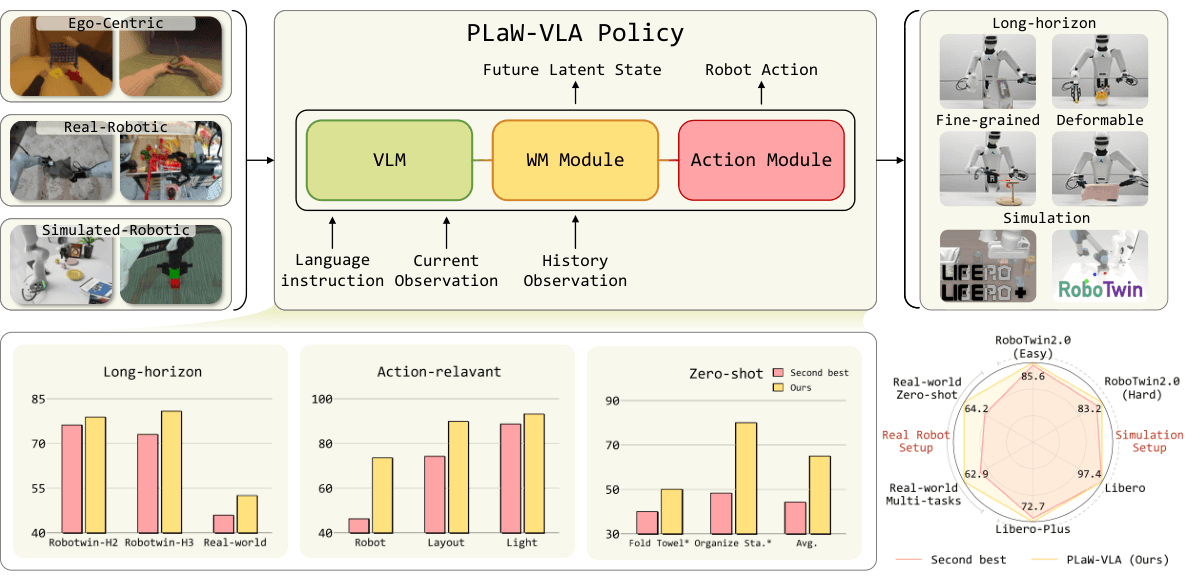
PLaW-VLA, short for Predictive Latent World Modeling for Vision-Language-Action Policies, adds predicted future representations to the information available to a robot policy. Rather than reconstructing a future video, it predicts features in the representation space of a frozen V-JEPA 2 encoder. An action expert then uses those features alongside the current scene, observation history, and language instruction.
This tutorial draws on the original paper, project page, and RainyRobo/PLaW-VLA repository. Run the examples on your own experiment machine, from the PLaW-VLA repository root.
Release status checked on October 12, 2026: training code, converters, and LIBERO evaluation are public, but the official pretrained PLaW-VLA checkpoint is pending release. The current quickstart loads public π₀.₅ foundation weights and initializes the world-model modules afresh. Completing that workflow therefore differs from reproducing the paper's complete Stage I–II pretrained policy.
1. Understand what the future prediction provides
A vision-language-action policy turns images, an instruction, and robot state into actions. A reactive policy relies primarily on what it can observe now. In a multi-step task, however, the same-looking scene can mean different things depending on what happened earlier. Closing the gripper before a grasp and opening it after placement are opposite decisions that may occur around similar object arrangements.
Observation history gives the model evidence about previous interactions. Future prediction adds an estimate of how the task might evolve. As an intuitive example, features corresponding to a lowered hand and an object inside a box could help a policy complete placement. This is an explanation of the intended mechanism, rather than a claim that the model outputs a readable sentence or a photorealistic image.
Three terms will appear throughout the tutorial. A latent is an encoder-produced feature vector. An action chunk contains targets for multiple future times. The end-effector, or EEF, is the robot's working endpoint, such as its gripper. LIBERO provides simulated manipulation tasks with a Franka robot, making it possible to study the complete pipeline without buying robot hardware.
PLaW-VLA does not introduce an explicit search over many candidate action sequences in the manner of a conventional planner. Its latent predictor conditions on observation history and task context; the action model then consumes the predicted features. Do not assume that each future query represents a separate action candidate being simulated.
2. Architecture: three experts with structured attention

The model uses a Mixture-of-Transformers architecture. A PaliGemma-based vision-language expert processes current multi-view observations and the instruction to produce semantic context. A latent world-model expert combines that context with historical features to predict future features. An action expert produces continuous action sequences using the semantic context, historical latents, and predicted future latents.
The frozen V-JEPA 2 encoder defines the target space for prediction. Keeping this encoder fixed stabilizes the feature targets during training. Learnable future queries correspond to future prediction steps and can be processed in parallel. There is no requirement to decode each prediction into pixels before producing actions.
The information flow is easiest to follow as a pipeline:
Current multi-view RGB + instruction -> vision-language context
Observation history -> frozen V-JEPA 2 -> history latents
Context + history + future queries -> predicted future latents
Context + history + predicted future -> action expert -> action chunk
Action chunk -> output transforms -> absolute EEF targets -> controller
Structured causal attention controls which token groups can exchange information. For a beginner, the crucial distinction is that actual future observations provide training targets only. At inference, the policy receives observations available up to the current time. Accidentally putting future frames into a client's history would invalidate the evaluation, even if the resulting rollout looked excellent.
3. Training objectives and branch dropout
The world-model objective aligns predicted future features with features extracted from actual future demonstration frames. It uses mean squared error, with stop-gradient applied to the target representation. The action expert learns continuous chunks through flow matching: it learns the vector field needed to transform noisy action samples into suitable action sequences.
During joint robot-policy training, both objectives contribute. The paper also uses world-model branch dropout with probability 0.3. On a dropped batch, historical and predicted latent tokens from that branch are omitted from action conditioning, and the world-model loss is disabled. The action-generation loss remains active. This encourages the policy to retain useful behavior when predictive context is unreliable.
A declining latent loss is not sufficient evidence of better control. Feature prediction can improve while the robot still releases an object too early or sends incorrectly scaled commands to its controller. Watch rollouts and task metrics alongside training curves; they measure different parts of the system.
4. Prepare the machine and Python environments
The repository installation instructions specify Linux x86_64, an NVIDIA GPU with a CUDA 12.8-compatible driver, and Python 3.12 for training. FFmpeg handles video decoding, while EGL and OpenGL libraries support simulator rendering. Plan storage for downloaded assets, datasets, and complete checkpoint directories.
The repository does not provide a universal minimum GPU specification that guarantees every recipe will fit. A single GPU's feasibility depends on its memory and the selected training settings. Begin by checking the driver and installing system dependencies:
nvidia-smi
sudo apt-get update
sudo apt-get install -y git ffmpeg libgl1 libegl1 libglib2.0-0
Install uv using its official installation guide. Then create the root environment:
git clone https://github.com/RainyRobo/PLaW-VLA.git
cd PLaW-VLA
git submodule update --init third_party/libero
GIT_LFS_SKIP_SMUDGE=1 uv sync --python 3.12 --frozen
bash scripts/setup/install_transformers_patch.sh
The frozen dependency lock helps keep the environment consistent with the repository. The Transformers patch is part of the prescribed setup; installing the standard package alone does not replace it. If the system Python lacks development headers, use uv's managed Python:
uv python install 3.12
UV_PYTHON_PREFERENCE=only-managed GIT_LFS_SKIP_SMUDGE=1 \
  uv sync --python 3.12 --frozen
bash scripts/setup/install_transformers_patch.sh
LIBERO's simulator client runs in a separate Python 3.8 environment. Training and serving remain in the root Python 3.12 environment:
uv sync --project examples/libero --python 3.8 --frozen
.venv/bin/python -c "import torch; print(torch.cuda.is_available())"
Keeping these environments separate prevents simulator dependencies from colliding with the training stack. If CUDA availability prints False, resolve that problem before downloading a large corpus or launching a training job.
5. Start with direct LIBERO fine-tuning
The quickstart prepares the foundation checkpoint, facebook/vjepa2-vitl-fpc64-256, tokenizer, prepared LIBERO EEF dataset, and matching normalization statistics. It is the most approachable entry point when your goal is to understand training and serving rather than recreate the complete pretraining corpus.
STAGE3_BASE_SOURCE=pi05 \
NUM_GPUS=8 EXP_NAME=libero_finetune \
  bash scripts/train/run_stage3_libero_quickstart.sh
This example pins pi05 explicitly so the initialization source will remain stable after the official PLaW-VLA checkpoint is released. The README uses auto, which currently resolves to π₀.₅ but is intended to select the complete PLaW-VLA checkpoint after release. Record the resolved source printed by the launcher when comparing experiments.
The default Stage III recipe uses 50,000 optimization steps, a global batch of 256, 10,000 warmup steps, and checkpoint saves every 5,000 steps. With eight processes, the stated global batch corresponds to 32 samples per process. NUM_GPUS must match the visible device count and divide the global batch size.
For an initial pipeline check, use a separate experiment with a small budget:
STAGE3_BASE_SOURCE=pi05 NUM_GPUS=1 EXP_NAME=libero_smoke \
  bash scripts/train/run_stage3_libero_quickstart.sh \
  --batch-size 1 --num-train-steps 20 --save-interval 10 \
  --no-wandb-enabled
This is a smoke run. It tests whether assets load, batches can be processed, and checkpoints can be written. It does not reproduce benchmark quality and does not guarantee sufficient VRAM on every GPU. PyTorch DDP replicates the full model and optimizer on each device; increasing the number of processes does not automatically split a model across GPU memories.
The full experiment saves checkpoints under:
checkpoints/stage3_finetuning_libero/libero_finetune/<step>/
Keep the entire step directory, including weights, saved assets, and training state. To resume, preserve the original source, process count, batch size, and any overrides:
STAGE3_BASE_SOURCE=pi05 NUM_GPUS=8 EXP_NAME=libero_finetune \
  bash scripts/train/run_stage3_libero_quickstart.sh --resume
If the original job disabled logging or changed another option, repeat that option during resume. The pretraining guide describes the checkpoint-loading modes and handoff rules.
6. Understand the complete three-stage route
Stage I uses visual sequences from InternData-A1, AgiBotWorld, RoboTwin, LIBERO, and EgoDex. Stage II uses the four robot sources with action labels; EgoDex contributes action-free video only to Stage I. The converted pretraining mixture is not distributed, and the repository notes that matching the exact paper mixture additionally requires the author-verified source manifest.
The following commands therefore assume you have already acquired, converted, and validated the data according to the data guide. Creating empty directories does not satisfy that prerequisite, and the wrappers do not automatically acquire the complete five-source corpus.
export DATA_ROOT="$PWD/data/pretrain"
NUM_GPUS=8 EXP_NAME=stage1_world_model \
  bash scripts/train/run_stage1_world_model_pretraining.sh

NUM_GPUS=8 STAGE1_EXP_NAME=stage1_world_model EXP_NAME=stage2_joint \
  bash scripts/train/run_stage2_pretraining.sh

NUM_GPUS=8 STAGE2_EXP_NAME=stage2_joint EXP_NAME=libero \
  bash scripts/train/run_stage3_finetuning_libero.sh
| Stage | Objective | Steps | Global batch |
|---|---|---|---|
| I | Video-based latent prediction; train LWM only | 100,000 | 512 |
| II | Joint future prediction and action learning | 100,000 | 256 |
| III | LIBERO task adaptation | 50,000 | 256 |
Before Stage II, compute normalization statistics using the canonical training transforms:
.venv/bin/python scripts/train/compute_norm_stats.py \
  --config-name stage2_pretraining --batch-size 32
Converter-level meta/stats.json describes raw stored features and does not replace transformed training statistics. Recompute them when the data selection or action convention changes. The default temporal recipe uses six history frames including the current frame, six future frames spaced 0.2 seconds apart, and actions at 0.1-second intervals. Preserve that temporal configuration across checkpoint handoffs.
7. Keep the action contract consistent
A single-arm canonical EEF representation contains position, a scalar-first quaternion ordered qw, qx, qy, qz, and one gripper value: eight dimensions in total. Stage III stores absolute EEF targets, but its training transforms express each target relative to the same current robot state. The second target is not a delta from the first target.
At inference, output transforms reconstruct absolute targets using that same reference state. The server returns timestamped physical EEF targets. The LIBERO client interpolates them, compares them with the live pose, and converts the pose error into a robosuite OSC command. An OSC_POSE controller consumes normalized commands; an absolute eight-dimensional target cannot simply be sent into it unchanged.
Gripper conventions require equal care. Physical width, open fraction, and signed controller commands are distinct representations. The raw RLDS converter produces signed commands and requires a matching custom configuration. It is not a drop-in replacement for the canonical EEF dataset used by the Stage III recipe. The normalization guide explains the checkpoint assets and representation contract.
This boundary matters when moving to another simulator or a real robot. The learned policy can remain unchanged while the observation and execution adapters change, but those adapters must preserve units, orientation conventions, timing, and gripper semantics.
8. Run inference through a server and client
In the first terminal, point the policy server at a checkpoint you actually created. The example uses step 30000, which is the LIBERO checkpoint reported in the paper even though the scheduled training budget is 50,000 steps.
.venv/bin/python scripts/serve/serve_policy.py \
  --env LIBERO --port 8001 policy:checkpoint \
  --policy.config=stage3_finetuning_libero \
  --policy.dir=checkpoints/stage3_finetuning_libero/libero_finetune/30000
Wait for the listening message. In a second terminal, first evaluate one task with a few trials to confirm rendering, communication, and action execution:
MUJOCO_GL=egl uv run --project examples/libero --frozen \
  python examples/libero/main.py \
  --task-suite-name libero_spatial --seed 42 \
  --task-ids 0 --num-trials-per-task 3 --record-video all
If you only ran the smoke experiment, use its actual step 10 or 20 directory instead. Such a checkpoint is useful for exercising the mechanism but is unlikely to produce meaningful task success. Three trials on one task are also too small a sample for model-quality conclusions.
Once the pipeline works, evaluate all four supported suites:
for suite in libero_spatial libero_object libero_goal libero_10; do
  MUJOCO_GL=egl uv run --project examples/libero --frozen \
    python examples/libero/main.py \
    --task-suite-name "$suite" --seed 42 --record-video failure
done
libero_10 is the suite commonly labeled LIBERO-Long in paper tables. By default, the client runs 50 trials per task, with 10 tasks per suite. For a meaningful comparison, repeat across three evaluation seeds and record your selected seeds, initialization source, checkpoint step, and recipe changes. A single seed-42 run does not match the paper's three-seed protocol.
Failed-rollout videos are written to results/libero/videos by default. The LIBERO evaluation guide also covers batch scheduling and checkpoint sweeps. Eager execution is the server default. Start there so first-run compilation latency does not obscure simulator or connection problems.
9. Interpret the reported results
| Method | Spatial | Object | Goal | Long | Average |
|---|---|---|---|---|---|
| π₀.₅ | 98.8 | 98.2 | 98.0 | 92.4 | 96.9 |
| PLaW-VLA | 98.9 | 99.0 | 97.1 | 94.6 | 97.4 |
Paper Table 1 reports a 0.5 percentage-point average gain and a 2.2-point Long gain. Goal is lower than the backbone, so the result should not be described as improvement on every suite. These are author-reported measurements, not a reproduction performed for this tutorial.
The paper separately reports 72.7% task-weighted zero-shot success on LIBERO-Plus. On RoboTwin Hard Horizon III, success increases from 67.4% to 79.2%, a gain of 11.8 percentage points. That larger gain belongs to RoboTwin, not LIBERO. Source: Experiments.
Replacing V-JEPA 2 with Cosmos VAE produces 70.93% on LIBERO-Plus, 1.77 points below the full model. Masking all predicted future states at inference lowers LIBERO success to 93.05%. These ablations support the role of the representation space and future conditioning within the tested setup; they do not establish that every robot will benefit equally. Source: Table 4.

The real-world experiment reports normalized task progress, which differs from binary simulation success. A robot that completes three of four stages can receive substantial progress credit while failing a strict whole-task criterion. Always compare metric definitions before putting simulation and hardware results on the same chart.
10. Troubleshoot and plan the next experiment
For EGL errors, check the GPU driver and rendering libraries first. The evaluation guide permits MUJOCO_GL=glx on systems using an X display. For connection failures, verify that the server is listening and that host and port match. If inference returns outputs but the robot moves incorrectly, inspect normalization assets, quaternion order, and gripper conventions before changing the model architecture.
When action loss falls without better success, inspect videos by stage: approach, grasp, transport, and release. Counting failure modes helps distinguish perception problems from controller conversion errors or missing recovery demonstrations. Keep datasets, execution adapters, seeds, and training budgets fixed when comparing policies; otherwise, an apparent gain may have multiple possible causes.
A useful first milestone is a valid checkpoint, a running policy server, and a saved rollout. The next is a complete suite evaluation with recorded provenance. Those milestones give you a sound basis for deciding whether to invest in full pretraining or hardware adaptation. Predictive context can help a policy track progress, while data quality and a consistent execution contract remain essential to successful manipulation.