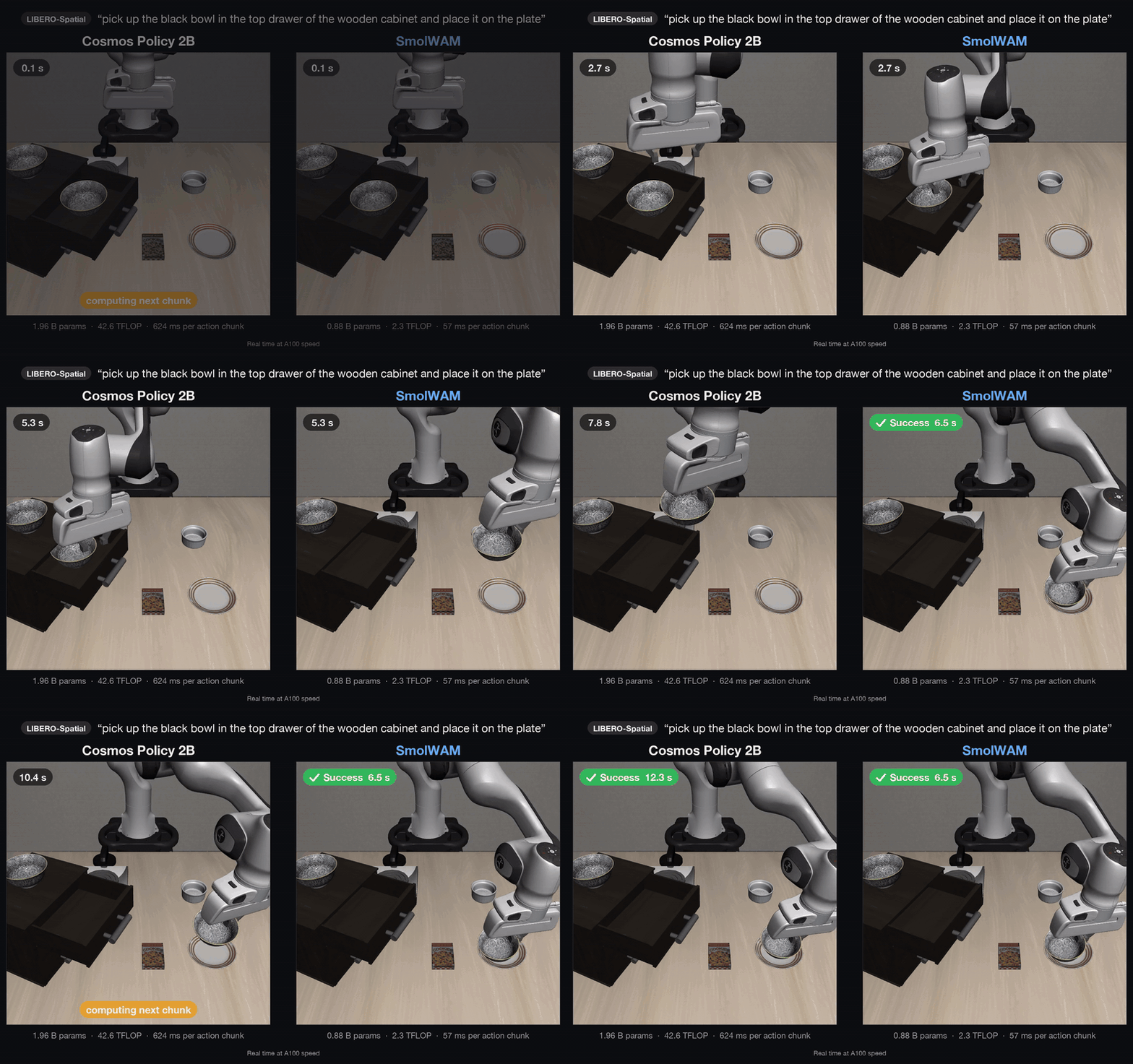
A robot policy usually receives camera images and a language instruction, then returns actions. SmolWAM also predicts what both camera views will look like after the robot executes those actions. It preserves this future-prediction capability in a network of approximately 0.88 billion parameters, without running the original large video model interface for every control query.
The SmolWAM repository reports 382 successful episodes out of 400, or 95.5%, on LIBERO. One query generates a chunk of 16 actions in approximately 57 ms, with 2.36 GiB peak GPU memory on an NVIDIA A100, batch size one, bf16, and cached text features. The frequently repeated “2.4 GB VRAM” description is therefore more precisely approximately 2.4 GiB for inference. It is neither the training memory requirement nor a promise of A100 latency on every small GPU.
This tutorial takes you through installation, sample inference, a simulated episode, evaluation, and training. The benchmark figures are the authors' published results. Commands have been checked against the released source; this article does not claim that vnrobo independently reran the full benchmark.
1. The idea: preserve the future, simplify the interface
The original research is SmolWAM: A Latent World-Action Model for Robotic Manipulation on Edge Devices, by Timi Owolabi, Hikmah Olawore, Frances Adelakun, and Ayotomiwa Oyewumi, released in October 2026. The project identifies it as work for the NeurIPS 2026 Workshop on Robot Learning with World Models.
VLA means Vision-Language-Action: visual observations and language instructions inform robot actions. A world-action model, or WAM, additionally represents the future observations associated with those actions. For a command such as placing a bowl on a plate, the model jointly predicts how to move and what the resulting scene should resemble.
SmolWAM inherits Cosmos Policy rather than learning a new foundation model from scratch. Its teacher uses a video diffusion backbone with an inference interface designed around video generation. That interface includes expensive clip encoding, long token sequences, and repeated denoising passes. The central question is how much of this machinery robot control actually needs.
The team retains pretrained knowledge, rebuilds the interface, prunes depth, and uses distillation to recover behavior. If you are familiar with LeRobot, do not confuse SmolWAM with SmolVLA. Our SmolVLA training guide covers a different compact policy. Here, predicting future visual latents remains part of the model's output.
2. Architecture in beginner-friendly terms
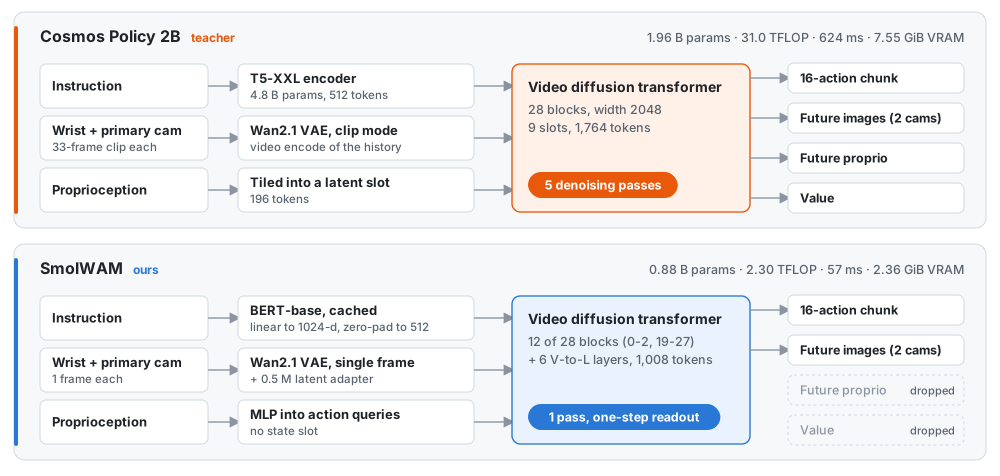
Source: assets/architecture.svg. Use this illustration to understand the components. Its teacher label shows 31.0 TFLOP; the current benchmark record used below reports 42.6 TFLOP for total teacher inference cost.
There are five useful architectural ideas to understand before running anything:
- Encode individual images. Each camera contributes its current frame, encoded by the Wan2.1 VAE. A roughly 0.5-million-parameter adapter maps these single-frame latents into the space expected by the pretrained trunk. Matching tensor dimensions alone would not guarantee matching latent distributions.
- Cache language features. BERT-base replaces the large T5-XXL language path. Projected features are zero-padded to 512 context positions, and six vision-to-language layers allow instruction features to interact with visual inputs.
- Retain selected transformer blocks. The model keeps blocks 0–2 and 19–27, twelve of the teacher's twenty-eight. This is a specific validated selection, not an instruction to remove arbitrary layers.
- Use state-conditioned action queries. Robot proprioception conditions 28 learned queries through an MLP. These replace the teacher's 196-token action frame while maintaining the relevant positional structure.
- Read actions and future latents in one pass. The network outputs both together. It does not need to decode a future RGB image before producing an action chunk.
Padding deserves attention. A zero-valued context position can still affect the denominator of an attention softmax. Removing apparently empty tokens may therefore change the computation, even though the remaining features look identical. When adapting pretrained models, preserving behavior involves more than making the weights load successfully.
Start with released weights before budgeting for a training GPU. Establishing that the API, simulator, and observation pipeline work gives you separate checkpoints for troubleshooting. It also prevents spending training time on an environment that cannot yet evaluate the resulting policy.
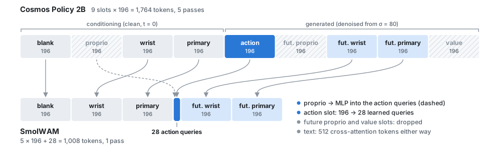
Source: assets/tokens.svg. The compact sequence contains a blank frame, two current camera frames, two future camera frames, and action queries: 5 × 196 + 28 = 1,008. The 512 language context positions belong to cross-attention and should not be confused with this trunk sequence count.
A latent is a compressed representation rather than a directly viewable image. You supply ordinary RGB arrays to the public API, but the model processes encoded visual features internally. Decoding predicted latents back into RGB is useful for inspection; it adds work beyond the default action-serving path.
3. Install in a clean Python environment
The package requires Python 3.10 or newer and PyTorch 2.5 or newer. It supports CUDA, Apple silicon through MPS, and CPU execution. Supporting a backend does not imply identical speed or memory behavior across backends. The headline latency was measured on an A100.
Download a source archive without needing Git operations:
curl -L https://github.com/iitimii/SmolWAM/archive/refs/heads/main.tar.gz \
  -o SmolWAM-main.tar.gz
tar -xzf SmolWAM-main.tar.gz
cd SmolWAM-main
python3 -m venv .venv
source .venv/bin/activate
python -m pip install --upgrade pip
python -m pip install -e .
Run these commands on your own experiment machine. For reproducibility, record the download date, source version, package versions, and GPU model. An archive of main can change over time. A clean virtual environment also makes dependency failures easier to identify than installing into an existing robotics environment with unrelated packages.
Check what PyTorch can actually access:
python -c "import torch; print(torch.__version__); print('CUDA:', torch.cuda.is_available()); print('MPS:', torch.backends.mps.is_available())"
If your NVIDIA machine reports CUDA unavailable, inspect the driver and installed PyTorch build before proceeding. Physically owning a GPU does not prove this Python process can use it. Likewise, this check does not establish whether a headless server can render the simulator; rendering is a separate dependency boundary.
The release lives at timiiowolabi/SmolWAM on Hugging Face. First use downloads approximately 3.5 GB of fp32 policy weights, a text cache, and approximately 0.5 GB of Wan2.1 VAE weights. Download size, disk cache, system RAM, and GPU memory describe different resources. Do not size the entire machine from the inference VRAM figure alone.
4. Run sample inference before installing simulation
The official quickstart includes a real LIBERO observation. You do not need to invent random input tensors or collect a dataset for your first inference call:
python examples/quickstart.py --device cuda --dtype bf16
Use the appropriate alternative on Apple silicon or a CPU machine:
python examples/quickstart.py --device mps --dtype fp32
# Alternatively:
python examples/quickstart.py --device cpu --dtype fp32
Choose the command matching your backend. The script warms up the model and prints the action shape and timing breakdown. Expect (16, 7): sixteen timesteps, each with six end-effector delta components and one gripper command. These are not sixteen joint angles and are not universal motor commands ready for an arbitrary robot.
The policy API implementation expects the following observation:
| Key | Meaning | Check before passing data |
|---|---|---|
primary_image |
Third-person RGB camera | Upright (H, W, 3) uint8 array |
wrist_image |
Wrist RGB camera | Correct orientation and RGB ordering |
proprio |
Nine-dimensional robot state | Two gripper joints, end-effector position, quaternion |
For a small API experiment using valid bundled data, run this from the extracted repository root:
python - <<'PY'
import sys
sys.path.insert(0, 'examples')
from quickstart import load_sample
from smolwam import SmolWAM

obs, instruction = load_sample()
policy = SmolWAM.from_pretrained(
    'timiiowolabi/SmolWAM', device='cuda', dtype='bf16'
)
actions = policy.predict_action(obs, instruction)
print(actions.shape)
print(policy.last_timing)
PY
The wrapper normalizes proprioception and unnormalizes actions using release statistics. Porting another robot's data therefore requires checking representation, units, coordinate conventions, and training distribution. A vector containing nine numbers is not automatically compatible just because its shape matches.
5. Install LIBERO and save one rollout
Use the project's LIBERO installation script, rather than choosing the newest simulation packages independently:
bash scripts/install_libero.sh
python examples/libero_rollout.py \
  --suite libero_10 --task 2 \
  --device cuda --dtype bf16 \
  --out outputs/rollout.mp4
The installation pins robosuite 1.4.0 and MuJoCo 3.3.2, and installs libero==0.1.1 through the prepared dependency path. Object assets of approximately 0.4 GB download on first use. The package handles LIBERO path configuration and selects EGL rendering on Linux or CGL on macOS.
Two separate checks matter: whether the program ran, and whether the environment reported task success. A video of an arm moving is evidence of activity, not necessarily successful manipulation. The rollout example reports success or failure, step count, and query timing, then saves an MP4 for inspection.
The controller observes, predicts sixteen actions, executes that chunk, and obtains another observation. The episode is closed loop across chunks, while each chunk executes open loop. Keep this distinction in mind when interpreting speed. Simply executing eight actions before querying again changes the temporal contract; it is not a validated drop-in method for improving reactivity.
LIBERO camera images have a rendering orientation convention that needs correction. The helper policy_observation(env_obs) handles this. If you write your own environment loop, use that helper rather than passing raw simulator arrays directly and accidentally giving the policy upside-down images.
6. Evaluate progressively and interpret the results
Begin with a small protocol to catch missing assets, rendering failures, or observation errors:
python -m smolwam.eval_libero \
  --protocol smoke --out outputs/eval_smoke.json
python -m smolwam.eval_libero \
  --protocol screen --out outputs/eval_screen.json
python -m smolwam.eval_libero \
  --protocol full --out outputs/eval_full.json
The experiment guide defines twelve smoke episodes, sixty screening episodes, and four hundred full-protocol episodes. Full evaluation covers four suites, ten tasks per suite, and ten trials per task, using seed 195 and fixed initial states. Training seed is a separate setting; do not replace one with the other when documenting reproduction.
| LIBERO suite | SmolWAM | Teacher comparison |
|---|---|---|
| Spatial | 99.0% | 97.0% |
| Object | 100.0% | 100.0% |
| Goal | 94.0% | 99.0% |
| Long | 89.0% | 97.0% |
| Overall | 95.5% | 98.2% |
Sources: the full evaluation record and repository comparison table. Teacher suite results originate from an earlier evaluation pipeline, while the original Cosmos Policy publication reports 98.5%. Preserve that provenance rather than silently treating all teacher figures as interchangeable.
The authors report a 95% Wilson interval of 93.0–97.1% for 382 successes out of 400. A high overall score does not mean every task achieves at least 95%. Long-horizon performance is the clearest weakness. If your intended application contains multiple sequential subgoals, failure videos and per-task records deserve more attention than a single average.
Measure inference cost in a separate process:
python -m smolwam.bench --out outputs/bench.json
The A100 efficiency record reports approximately 2.30 TFLOP for SmolWAM and 42.61 TFLOP for the teacher, approximately an 18.5-fold reduction. Run latency measurements with the GPU otherwise idle. Parallel evaluation workers introduce contention, so their timings are not comparable to an uncontended benchmark.
Approximately 282 actions per second is chunk throughput converted into action count. The model produces only about 17.7 new chunks per second, and chunks execute open loop. This is not a claim that the robot processes 282 fresh camera observations every second.
7. Inspect the predicted future
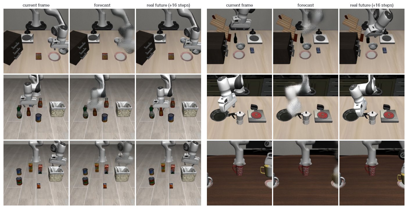
Source: assets/dreams.jpg. Predicted images illustrate the model's forecast; their visual quality should be evaluated separately from manipulation success.
Run the world-model example:
python examples/world_model.py \
  --device cuda --dtype bf16 \
  --out outputs/world_model.png
The example requests return_future=True, then calls decode_future(...). Its output places the current view beside the forecast, with wrist and primary cameras on separate rows. This forecast represents the view sixteen steps ahead. It is not a dense video of all sixteen intermediate frames.
The world-model metrics record evaluates ninety-six held-out contexts. Latent L1 falls from 0.133 for copying the current frame to 0.101 for SmolWAM. Primary-camera optical-flow endpoint error falls from 1.63 to 1.43 pixels. Primary LPIPS, however, is 0.128 versus 0.115 for the copy baseline, so the model does not improve every image metric.
A useful interpretation is that the forecast contains motion information while texture can remain blurry. Predicting roughly where the arm will move and reproducing its exact appearance are different capabilities. Neither a visually pleasing forecast nor a low image error alone establishes reliable planning or collision avoidance.
8. Reproduce training with the released recipe
Light inference does not imply light training. The training script reproduces the release on one A100 with 40 GB memory. The full pipeline takes approximately five hours in the reported setup; optimizer training accounts for 3.6 hours.
python -m pip install -e '.[train]'
python -m pip install -U huggingface_hub
bash experiments/train_smolwam.sh
The script downloads nvidia/LIBERO-Cosmos-Policy demonstrations, builds a latent bank, fits the adapter, caches language features, creates teacher targets, trains the student, and exports a release. It starts from 1,700 successful demonstrations and samples observations every fourth step to produce 68,830 rows. The short training time relies on existing robot data and a pretrained teacher.
| Setting | Released recipe |
|---|---|
| Optimizer | AdamW |
| Batch size | 32 |
| Training steps | 5,000 |
| Inherited trunk learning rate | 2e-5 |
| New module learning rate | 1e-4 |
| Initial layout | 1,764 tokens for 1,000 steps |
| Final layout | 1,008 tokens for the remaining 4,000 steps |
| CUDA precision | bf16 |
Source: the released training configuration. The curriculum allows the student to recover after pruning before learning the compact layout. Making both changes simultaneously introduces a larger distribution shift. A falling training loss alone would not prove that the robot can recover correct closed-loop behavior.
The training implementation combines L1 supervision from demonstration actions and future latents with teacher action and future-latent targets. Future proprioception and value terms have weight 0.1 while those slots exist. The deployable best.pt checkpoint is selected by validation action L1 during the compact phase; last.pt also stores optimizer state for resuming.
After the pipeline finishes, test and evaluate the exported directory:
python examples/quickstart.py --model runs/smolwam/release
python -m smolwam.eval_libero \
  --model runs/smolwam/release \
  --protocol full --out outputs/retrained_full.json
Validation action error is a checkpoint-selection signal, not a substitute for full task success. Claiming reproduction requires evaluating your own exported checkpoint and reporting its actual result and conditions. More training is not automatically better: the reported extended-training variant reaches 94.2% full success after an additional 7,500 steps.
9. Troubleshooting and deployment boundaries
If sample inference runs out of GPU memory, inspect other GPU processes, the selected dtype, and whether the instruction is cached. An unseen instruction loads BERT for live encoding, potentially changing memory and latency. Decoding future images adds more work as well. The 2.36 GiB default-path measurement is not a guarantee that every API path fits the same memory budget.
If quickstart works but simulation fails, investigate rendering, LIBERO assets, and pinned dependency versions. If simulation runs but the policy repeatedly fails, check camera orientation, proprioception ordering, normalization, task selection, and initial state. These boundaries help diagnose the failing component without reinstalling the entire stack unnecessarily.
The release is evaluated on simulated LIBERO tasks with one training seed. It has not established performance on real robots or measured embedded-device throughput. The repository reports about 0.9 seconds per query on an M2 Pro, rather than the A100's 57 ms. Its INT8 ablation uses simulated weight quantization with bf16 kernels, which should not be presented as measured native INT8 deployment speed.
Code and checkpoint licensing also differ. The code is Apache-2.0, while the repository states that weights derived from Cosmos Policy use the NVIDIA One-Way Noncommercial License. Read the model card and applicable weight license when planning use; code licensing alone does not establish commercial rights to the checkpoint.
A practical learning sequence is to verify the sample (16, 7) output, inspect a single rollout, complete smoke evaluation, run the full protocol, and then reproduce training. Each stage supplies a different piece of evidence: a functioning API, a functioning simulator, a correct evaluation protocol, and a newly trained checkpoint with measured behavior.