ETH Zürich has made the Spring 2026 course Robot Learning: From Fundamentals to Foundation Models publicly accessible. The course is taught by Oier Mees, and the official page is available at cvg.ethz.ch/lectures/Robot-Learning. The homework repository is mees-robot-learning-course/ethz-course-2026.
What makes this course useful is not only the lecture recordings. It gives a structured route through the stack that beginners usually have to assemble manually: PyTorch, robot control, MDPs, imitation learning, reinforcement learning, generative policies, sequence modeling, world models, generalist robot policies and finally Vision-Language-Action (VLA) / foundation models for robotics.
If you have been following robotics RL basics, imitation learning, Diffusion Policy, or VLA models, this course can serve as the practical spine. This article explains the technical path: the paper ideas, the architecture of the assignments, how to install and train the code, how inference/evaluation works, and what results a beginner should expect.
The core idea: learn robot learning as a stack
Robot learning is easy to misunderstand as a model-selection problem. Pick Diffusion Policy, ACT, OpenVLA, π0, Gato, or the newest VLA and hope the robot becomes intelligent. In practice, the model is only one layer. You still need to understand state/action design, control loops, data distributions, reward design, offline datasets, rollout evaluation and inference latency.
The ETH course is valuable because it climbs this stack from first principles:
| Layer | Question to answer | Homework or paper example |
|---|---|---|
| Tensor and networks | How do tensors, autograd and training loops work? | HW1 PyTorch/Numpy, MNIST, GLU |
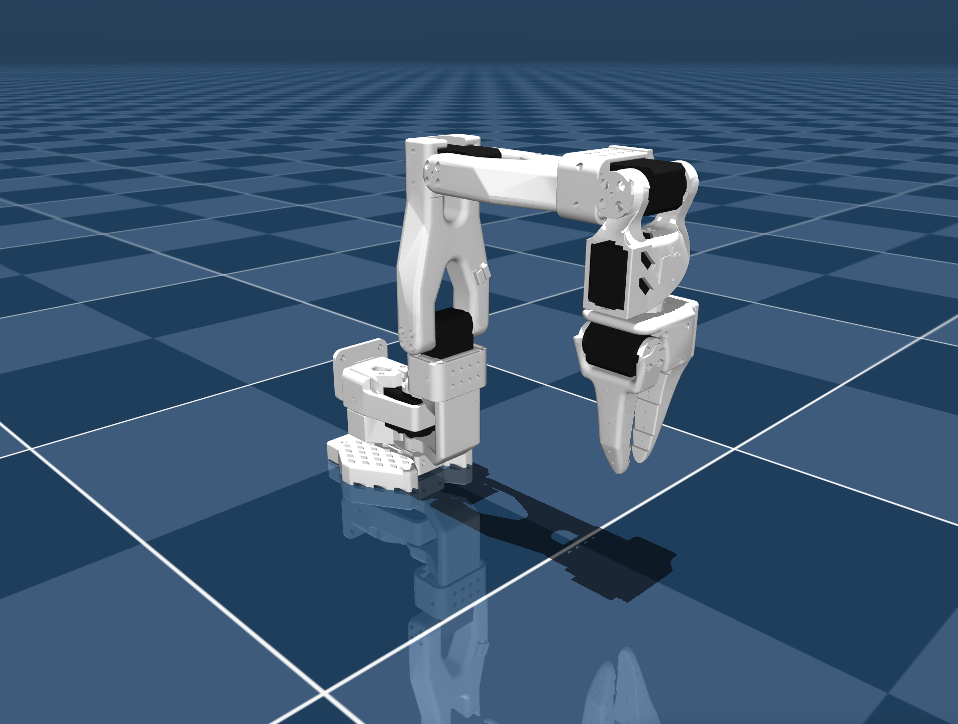
| Control and MDPs | What are robot states/actions, IK, PID and trajectories? | HW2 SO-100/SO-101 MuJoCo |
| Imitation learning | How do demonstrations become datasets and policies? | HW3 teleoperation, zarr, DAgger |
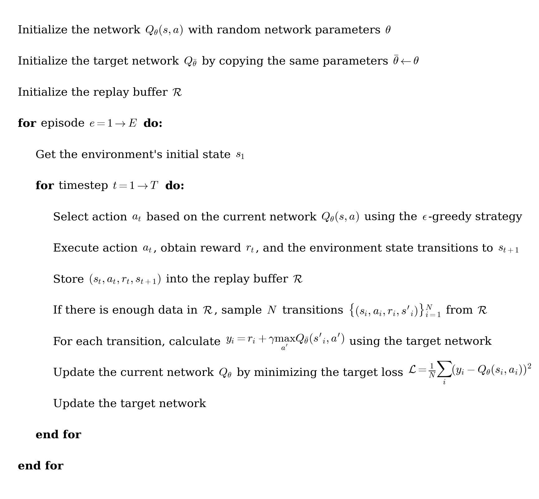
| Reinforcement learning | How does a robot learn from reward and interaction? | HW4 value iteration, DQN, PPO, SAC |
| Generative/sequence models | Why can actions be trajectories, tokens or denoising samples? | Diffusion Policy, Decision Transformer |
| Foundation models | How does one model combine vision, language and action? | Gato, π0.6, VLA papers |
The course does not start with a foundation model. It starts with a small arm in MuJoCo, where every failure is visible: inverse kinematics fails to converge, PID oscillates, reward shaping is wrong, the imitation policy overfits demonstrations, DQN becomes unstable, or PPO/SAC learns slowly. Once you have seen those failures, VLA papers become much easier to reason about.
Original papers and projects to read
The early control/RL weeks include papers such as Simple random search provides a competitive approach to reinforcement learning, Deep RL Doesn't Work Yet, and Curiosity-driven Exploration by Self-supervised Prediction. The shared lesson is pragmatic: deep RL is not magic. A simple baseline can be competitive if the benchmark is weak, and exploration does not appear automatically when reward is sparse.
The imitation learning week includes Causal Confusion in Imitation Learning, The Surprising Effectiveness of Representation Learning for Visual Imitation, and Transporter Networks. These papers explain why behavior cloning is more subtle than minimizing MSE from observation to action. A policy can latch onto correlated but non-causal features, validate well, then fail when lighting, camera viewpoint or object placement shifts.
The generative models week brings in Diffusion Policy and the paper Visuomotor Policy Learning via Action Diffusion. Diffusion Policy treats an action sequence as a sample from a distribution and generates actions through denoising. The authors report evaluation across manipulation benchmarks with an average improvement of about 46.9% over prior state-of-the-art baselines. If you read our Diffusion Policy deep dive, this week connects behavior cloning to generative action modeling.
The sequence modeling week uses Decision Transformer. Its key idea is to cast RL as conditional sequence modeling: input return-to-go, state and previous action tokens; output the next action. Instead of directly learning a Q-function or policy gradient, the model learns trajectories with a Transformer.
The generalist policy week uses Gato, a single Transformer that can process tasks such as Atari, captioning, chat and block stacking with one set of weights. This is an important conceptual bridge to VLA: observations, text and actions can all be represented as tokens in a shared sequence.
The VLA/foundation model week includes π*0.6: a VLA That Learns From Experience, where Physical Intelligence studies how VLA models can improve through real-world deployments using RL and advantage-conditioned policies. This connects large offline imitation models back to real experience.
Assignment architecture
The official repo currently has four main homework folders:
ethz-course-2026/
├── hw1_pytorch_tutorial/
├── hw2_robot_control_mdps/
├── hw3_imitation_learning/
└── hw4_reinforcement_learning/
HW1 is the PyTorch foundation. Students work through tensor basics, core operations, neural networks, MNIST training/test curves and GLU experiments. The point is not to train a large model. The point is to understand dtype, device placement, autograd, plotting, reproducibility and statistical significance.
HW2 uses an SO-100/SO-101 arm in MuJoCo. Students implement keypoints on a Lemniscate of Bernoulli, inverse kinematics with Damped Least Squares, quintic spline waypoint generation, PID control and a PPO policy for random waypoint tracking. The control loop is intentionally realistic: the policy outputs an action at 10 Hz, MuJoCo steps at 500 Hz, ctrl_decimation = 50, and reward depends on end-effector tracking error. The assignment states that a trained policy receives full score when Average final EE tracking error < 0.05.
HW3 is a modern imitation learning pipeline. Students teleoperate the SO-101 arm in simulation, store raw observations in zarr, compute actions as deltas between states, train a policy, evaluate success rate and use DAgger when the policy falls out of distribution. Exercise 1/2 uses ObstaclePolicy; exercise 3 becomes a multicube goal-conditioned task with MultiTaskPolicy, three colored cubes, randomized bin position and one-hot state_goal.
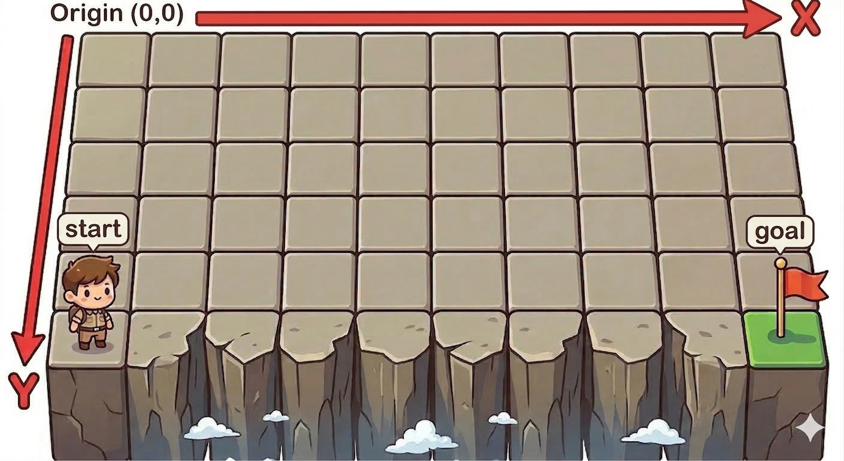
HW4 covers RL from tabular methods to continuous control: policy/value iteration on Cliff Walking, DQN on CartPole, PPO and SAC on SO100. The SO100 observation is a 19-dimensional vector containing joint positions, end-effector pose, target position and position error in the robot base frame. The action is a 6D vector in [-1, 1]^6, then linearly mapped to physical joint ranges.
Installation
Beginners should run each homework in a clean virtual environment. Several assignments are tested with Python 3.12 and use either uv or venv. For HW3:
cd hw3_imitation_learning
uv venv --python 3.12
source .venv/bin/activate
uv pip install -e .
Important dependencies include:
| Package | Purpose |
|---|---|
torch, torchvision |
neural networks, training loops, supervised policies |
mujoco, dm-control |
physics simulation and robot viewers |
gymnasium |
RL environment API |
stable-baselines3 |
PPO for HW2 |
tensorboard |
reward/loss curve visualization |
zarr |
demonstration dataset storage |
opencv-python |
frame processing and recordings |
On Linux, if the MuJoCo viewer fails with EGL/OpenGL issues, the HW2 installation guide recommends installing Mesa/EGL libraries such as libegl1-mesa-dev, libgl1-mesa-dri and libglvnd-dev. A simple smoke test is:
python scripts/interactive.py
For HW4, the SO100 MuJoCo stack can be smoke-tested headlessly:
python -c "from pathlib import Path; import numpy as np; from envs.so100_rl_env import SO100RLEnv; env=SO100RLEnv(xml_path=Path('assets/mujoco/so100_pos_ctrl.xml').resolve(), render_mode=None); obs,_=env.reset(seed=0); obs2,reward,term,trunc,info=env.step(np.zeros(env.action_dim, dtype=np.float32)); env.close(); print('OK ex3/ex4:', obs.shape, float(reward))"
If you are new to robotics, do not start with the VLA lecture. Start by opening the viewer, moving the robot, understanding qpos, qvel, data.ctrl and mj_step. Those variables are the physical interface that every policy eventually has to control.
Training path
In HW1, training is intentionally small: MNIST and GLU experiments. You are expected to show training and test loss curves, then discuss what they mean. This is important because robot learning is full of misleading single-number metrics; learning to read curves early is useful.
In HW2, PPO waypoint training begins only after the environment has an observation, action processing and reward. A typical flow is:
cd hw2_robot_control_mdps
python scripts/train.py --max_iterations 500 --save_checkpt_freq 50
tensorboard --logdir=logs --port=6006
During training, the policy receives robot/target observations, outputs normalized actions, the environment scales them to joint targets, MuJoCo advances the physics, and reward is computed from tracking error. If reward is too weak, learning is slow. If action limits are too broad, the arm may jitter or hit joint limits. If target sampling is narrow, the policy may look good but fail on new positions.
In HW3, imitation learning starts with data:
python scripts/configure_keys.py
python scripts/record_teleop_demos.py
python scripts/compute_actions.py
python scripts/train.py --state-keys state_ee_xyz state_gripper "state_cube[:5]" --action-keys action_ee_xyz action_gripper --policy obstacle
A beginner should pay attention to the action space. The action does not have to be absolute joint position. The repository encourages choosing a simpler action representation when helpful, such as end-effector deltas plus gripper action. The dataset can include keys such as state_ee_xyz, state_ee_full, state_joints, state_gripper, state_cube, state_obstacle and goal_pos. The multicube version adds original_pos_cube_red, original_pos_cube_green, original_pos_cube_blue and state_goal.
In HW4, DQN uses replay buffer, epsilon-greedy exploration and a target network; PPO uses clipped surrogate objective, value loss and entropy; SAC uses twin critics, entropy bonus and automatic temperature tuning. At the beginner level, the high-level comparison is enough:
| Algorithm | Action type | Reuses old data? | Main concern |
|---|---|---|---|
| DQN | discrete | yes, replay buffer | target network, overestimation |
| PPO | continuous or discrete | mostly on-policy | clipping, GAE, KL drift |
| SAC | continuous | yes, off-policy | entropy, twin Q, temperature |
Inference and evaluation
Inference for robot policies is not the same as generating a text answer. A policy outputs actions repeatedly at a control frequency, and each action changes the next observation. Evaluation must therefore be rollout-based.
HW2 random-target evaluation:
python scripts/evaluate_rand_targets.py --load_run=1 --checkpoint=500
This runs 10 episodes, each 2 seconds long, and prints final end-effector tracking error plus the average. The assignment target is Average final EE tracking error < 0.05. This is a good beginner metric because it directly measures whether the end effector reached the desired target.
HW3 imitation evaluation:
python scripts/eval.py --checkpoint <path_to_checkpoint.pt> --num-episodes 100 --headless
python student_eval/run_eval --exercise 1 --checkpoint <path_to_checkpoint.pt>
Exercise 1/2 scoring is success-rate based: 85% or above receives full score, with lower bands at 75%, 65%, 55% and 45%. The multicube task is much harder; the README notes that a success rate approaching 50% is already strong. That is an important robotics lesson: a multi-task goal-conditioned policy is harder not only because of model size, but because of data coverage, task ambiguity and distribution shift.
HW4 PPO/SAC evaluation:
python scripts/eval_ppo.py
python scripts/eval_ppo.py --play
python scripts/eval_sac.py
python scripts/eval_sac.py --play
The evaluation summary reports mean return, return standard deviation, min/max return, mean length and mean tracking error. When watching the GUI playback, look for three failure modes: oscillation around the target, hitting joint limits, and reward hacking where the return improves but the end-effector behavior is unstable.
Results and practical meaning
The course is not a new SOTA benchmark. Its value is that each assignment has a clear result that tells you whether you actually understand the layer you are working on:
| Part | Expected output | Healthy result |
|---|---|---|
| HW1 | loss curves, GLU discussion | understand train/test behavior and significance |
| HW2 IK/PID | robot tracking keypoints/Lemniscate | smooth motion with limited oscillation |
| HW2 PPO | average final EE error | below 0.05 |
| HW3 IL | success rate | 85%+ for exercise 1/2 is full score |
| HW3 multicube | goal-conditioned success rate | near 50% is strong |
| HW4 PPO/SAC | return and tracking-error summary | stable rollouts |
When this is connected to the larger papers, the progression becomes clear. Diffusion Policy addresses multimodal action distributions that MSE behavior cloning handles poorly. Decision Transformer reframes RL as sequence modeling. Gato shows that a single network can handle multiple modalities and embodiments through tokenization. π*0.6 brings VLA models back into a real-world improvement loop through experience and RL-style updates.
A 6-week beginner study plan
Do not try to finish all 12 weeks in one weekend. A practical self-study plan looks like this:
Week 1: Watch the introduction and complete HW1 tensor/PyTorch exercises. Goal: write a small training loop and interpret loss curves.
Week 2: Work through HW2 inverse kinematics, quintic splines and PID. Goal: understand workspace, joint space, Damped Least Squares and why the low-level control loop is faster than the policy loop.
Week 3: Train the HW2 PPO waypoint policy. Goal: use TensorBoard, understand reward, action scaling, checkpoints and evaluation.
Week 4: Complete HW3 single-cube imitation learning. Goal: collect clean demonstrations, compute actions, train ObstaclePolicy and evaluate success rate.
Week 5: Run DAgger and multicube. Goal: observe distribution shift directly, where a policy that works on the training distribution fails when obstacle, bin or cube placements change.
Week 6: Read Diffusion Policy, Decision Transformer, Gato and π*0.6. Goal: connect modern architectures to concrete failures you have already seen in the homework.
If you are working in a small lab, you can adapt the course to cheaper arms or even simulation-only experiments first. Preserve the interface: observation, action, dataset, training, inference and evaluation. That interface matters more than the exact robot.
Common beginner mistakes
The first mistake is jumping straight into VLA. VLA models are exciting, but if you do not know whether your robot action is a joint target, an end-effector delta or a gripper command, you cannot debug the policy.
The second mistake is collecting a lot of low-quality data. HW3 notes that if the teleoperator stands still for many seconds during recording, the dataset will contain many "do nothing" actions. The policy may then learn to be passive. Robotics data is not only about quantity; it is about coverage and action quality.
The third mistake is evaluating only a successful video. Always run many headless episodes, record success rate and tracking error, and inspect failure cases. A policy that fails 15% of the time can still look excellent if you only show the best rollout.
The fourth mistake is ignoring the difference between training and inference. During training, a policy may rely on randomization, exploration noise, replay buffers or teacher corrections. During inference, it has only the current observation and the checkpoint. Hidden assumptions show up quickly when deployed.
Conclusion
ETH Robot Learning 2026 is worth studying because it does not sell the story that foundation models solve robotics by themselves. It teaches the stack: tensors, control, MDPs, imitation learning, RL, generative policies, sequence models, world models and then VLA/foundation models. For beginners, that is the least confusing path. Each modern paper appears after you have already seen the concrete problem it tries to solve.
For the next step, continue with the LeRobot ecosystem, OpenVLA deep dives and whole-body VLA training pipelines. Concepts such as dataset schemas, action chunking, diffusion heads, policy rollouts and sim-to-real will become much easier to reason about.