Tại sao Behavior Cloning truyền thống thất bại?
Nếu bạn đã thử dạy robot bắt chước hành động con người (imitation learning), chắc hẳn bạn biết Behavior Cloning (BC) — cách tiếp cận đơn giản nhất: thu thập demonstrations, train supervised learning, predict action từ observation. Đơn giản, dễ implement, nhưng thất bại thảm hại trong nhiều scenario thực tế.
Vấn đề multimodal actions
Hãy tưởng tượng: bạn dạy robot đi vòng qua một vật cản. Người demo lần 1 đi vòng bên trái, lần 2 đi vòng bên phải — cả hai đều đúng. BC với MSE loss sẽ học gì? Trung bình của hai hướng — nghĩa là robot đâm thẳng vào vật cản.
Demo 1:  ← (vòng trái)     ✓ Đúng
Demo 2:  → (vòng phải)     ✓ Đúng
BC output: ↑ (trung bình)  ✗ Đâm thẳng!
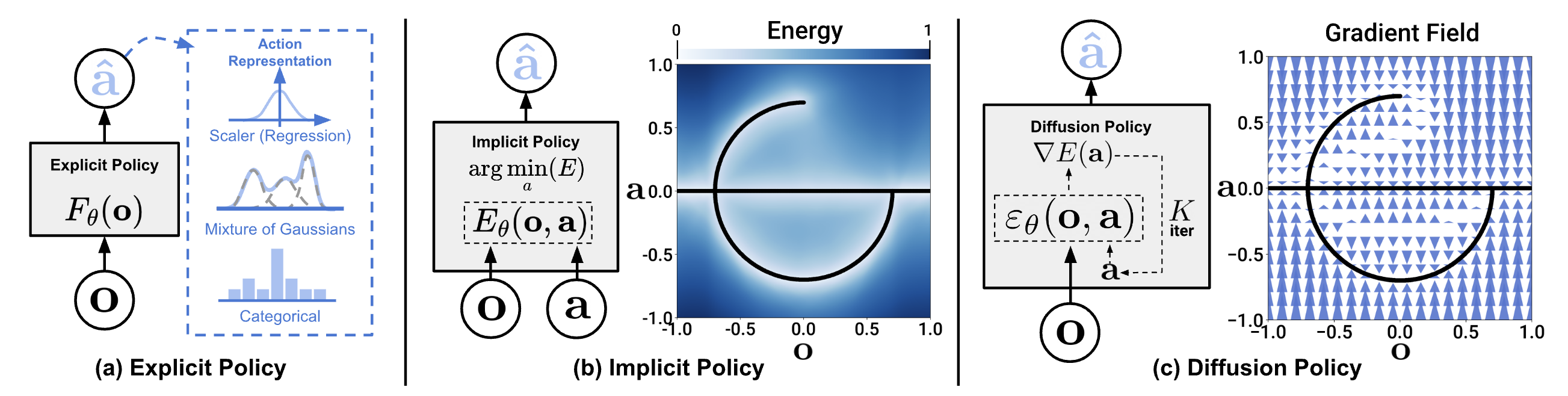
Đây là multimodal action distribution — khi cùng một observation có nhiều actions đúng. BC với Gaussian regression chỉ output 1 mode (mean), bỏ mất toàn bộ diversity trong data.
Compounding errors
Vấn đề thứ hai: mỗi prediction sai một chút, error tích lũy theo thời gian. Sau 50 steps, robot lệch hoàn toàn khỏi trajectory đã học. Đây là lý do BC hoạt động tốt trong simulation nhưng fail trên robot thật — real world luôn có noise và perturbations.

DDPM cơ bản: Forward noise và reverse denoising
Trước khi hiểu Diffusion Policy, cần nắm Denoising Diffusion Probabilistic Models (DDPM) — nền tảng của mọi diffusion models.
Forward process: Thêm noise dần dần
Cho một data point x₀ (ví dụ: một action trajectory), forward process thêm Gaussian noise qua T steps:
x₀ (clean action) → x₁ (ít noise) → x₂ → ... → x_T (pure noise)

Mỗi step: x_t = √(1-β_t) · x_{t-1} + √(β_t) · ε
Trong đó: ε ~ N(0, I), β_t là noise schedule
Sau T steps (thường T=100 hoặc 1000), x_T gần như hoàn toàn là Gaussian noise — không còn thông tin gì về x₀.
Reverse process: Denoise để sinh data
Reverse process học cách đi ngược — từ noise tạo ra clean data:
x_T (noise) → x_{T-1} → ... → x₁ → x₀ (clean action)

Mỗi step: x_{t-1} = μ_θ(x_t, t) + σ_t · z
Trong đó: μ_θ là neural network predict noise, z ~ N(0, I)
Neural network ε_θ(x_t, t) được train để predict noise ε đã thêm vào ở mỗi step t. Loss function đơn giản:
L = E[‖ε - ε_θ(x_t, t)‖²]
Điểm hay: model không predict action trực tiếp, mà predict noise cần loại bỏ. Qua nhiều bước denoising, action "hiện ra" từ noise — giống cách sculptor tạc tượng bằng cách bỏ đá thừa.
Tại sao diffusion models capture được multimodal distributions?
Khác với regression (chỉ output 1 giá trị), diffusion models học toàn bộ distribution của data. Mỗi lần sample, process bắt đầu từ random noise khác nhau, dẫn đến output khác nhau — tự nhiên capture được multiple modes.
Quay lại ví dụ đi vòng vật cản:
- BC: Luôn output trung bình → đâm thẳng
- Diffusion: Sample lần 1 → vòng trái. Sample lần 2 → vòng phải. Cả hai đều valid!
Diffusion Policy: Apply diffusion vào action space
Diffusion Policy (Chi et al., RSS 2023) là paper đầu tiên apply thành công diffusion models vào robot visuomotor policy learning. Ý tưởng cốt lõi: thay vì dùng diffusion để generate images, dùng nó để generate action trajectories.
Kiến trúc tổng quan
Observation (image + proprio)
        ↓
   Visual Encoder (ResNet / ViT)
        ↓
   Observation embedding (conditioning)
        ↓
   Conditional Denoising Network
   Input: noisy action chunk A_t^k + timestep k + obs embedding
   Output: predicted noise ε_θ
        ↓
   K denoising steps (DDPM hoặc DDIM)
        ↓
   Clean action chunk A_t^0 = [a_t, a_{t+1}, ..., a_{t+H}]
Điểm quan trọng: model predict cả chunk actions (ví dụ 16 actions liên tiếp) thay vì 1 action tại một thời điểm. Đây gọi là action chunking — giúp giảm compounding errors vì robot thực hiện cả đoạn trajectory mượt mà, không cần re-predict mỗi step.
Hai biến thể architecture
Paper đề xuất 2 kiến trúc cho denoising network:
1. CNN-based (1D temporal convolution):
# Simplified CNN-based Diffusion Policy
class ConvDiffusionUnet(nn.Module):
    """
    1D U-Net xử lý action sequence theo temporal dimension.
    Tương tự image diffusion U-Net nhưng 1D thay vì 2D.
    """
    def __init__(self, action_dim=7, obs_dim=512, horizon=16):
        super().__init__()
        # Observation conditioning via FiLM
        self.obs_encoder = nn.Linear(obs_dim, 256)
        # 1D U-Net with residual blocks
        self.down_blocks = nn.ModuleList([
            ResBlock1D(action_dim, 64),
            ResBlock1D(64, 128),
            ResBlock1D(128, 256),
        ])
        self.up_blocks = nn.ModuleList([
            ResBlock1D(256, 128),
            ResBlock1D(128, 64),
            ResBlock1D(64, action_dim),
        ])
        # Timestep embedding
        self.time_embed = SinusoidalPosEmb(256)
- Nhanh hơn, phù hợp real-time
- Tốt cho low-dimensional action spaces
2. Transformer-based (Time-series Diffusion Transformer):
# Simplified Transformer-based Diffusion Policy
class DiffusionTransformer(nn.Module):
    """
    Transformer xử lý action tokens + observation tokens.
    Attention mechanism giúp capture long-range dependencies.
    """
    def __init__(self, action_dim=7, obs_dim=512, horizon=16):
        super().__init__()
        self.action_embed = nn.Linear(action_dim, 256)
        self.obs_embed = nn.Linear(obs_dim, 256)
        self.transformer = nn.TransformerEncoder(
            nn.TransformerEncoderLayer(d_model=256, nhead=8),
            num_layers=6,
        )
        self.action_head = nn.Linear(256, action_dim)
- Flexible hơn, scale tốt hơn
- Tốt cho high-dimensional tasks và long horizons

Kết quả: Tại sao Diffusion Policy beats BC by 46.9%
Paper benchmark trên 12 tasks từ 4 robot manipulation benchmarks khác nhau. Kết quả ấn tượng:
| Task Category | BC (LSTM) | BC (Transformer) | IBC | BET | Diffusion Policy |
|---|---|---|---|---|---|
| Push-T | 49.1% | 51.2% | 45.3% | 60.1% | 88.5% |
| Robomimic (Can) | 78.3% | 82.1% | 71.6% | 75.4% | 96.2% |
| Robomimic (Square) | 52.1% | 55.4% | 44.2% | 48.7% | 84.8% |
| Real Robot (Push-T) | 35.0% | 38.2% | 30.1% | 42.3% | 72.1% |
| Average improvement | +46.9% |
Tại sao improvement lớn đến vậy?
-
Multimodal capture: Diffusion Policy tự nhiên xử lý được multimodal actions — khi data có nhiều cách giải quyết, model sample từ distribution thay vì lấy trung bình.
-
Action chunking + receding horizon: Predict cả chunk 16 actions, thực hiện 8 actions đầu, rồi re-plan. Giảm compounding errors và tạo smooth trajectories.
-
High-dimensional stability: Diffusion process ổn định hơn so với direct regression, đặc biệt khi action space lớn (bimanual: 14D+).
-
Training stability: Loss landscape mượt hơn nhờ predict noise thay vì predict action trực tiếp. Không cần careful hyperparameter tuning như IBC hay EBM-based methods.
Training chi tiết: Action horizon và observation conditioning
Action horizon và chunking
Diffusion Policy sử dụng 3 hyperparameters quan trọng:
Observation horizon (T_o): Số frames observation history = 2
Action horizon (T_a):      Số actions predict = 16
Action execution (T_e):    Số actions thực sự execute = 8

Timeline:
  t-1  t  |  t+1  t+2  ...  t+8  |  t+9  ...  t+16
  [obs ]  |  [execute these]      |  [predicted but discarded]
           ↑ re-plan tại t+8
Predict 16 nhưng chỉ execute 8, sau đó re-plan với observation mới. Phần "predicted but discarded" giúp model plan ahead — biết trajectory cần đi đâu sau 8 steps, nên 8 steps đầu sẽ smooth hơn.
Observation conditioning
Visual observations được encode bằng pre-trained ResNet hoặc ViT, sau đó condition vào denoising network qua FiLM conditioning (Feature-wise Linear Modulation):
# FiLM conditioning: obs ảnh hưởng đến denoising process
# tại mỗi layer của U-Net
gamma = self.gamma_layer(obs_embedding)  # Scale
beta = self.beta_layer(obs_embedding)     # Shift
features = gamma * features + beta        # Modulate
Cách này hiệu quả hơn concatenation vì obs embedding ảnh hưởng đến mọi layer của network, không chỉ input layer.
Code example với LeRobot
LeRobot của Hugging Face cung cấp implementation sẵn của Diffusion Policy. Đây là cách train và evaluate:
# Install LeRobot
pip install lerobot

# Train Diffusion Policy trên PushT task
python lerobot/scripts/train.py \
    --output_dir=outputs/train/diffusion_pusht \
    --policy.type=diffusion \
    --dataset.repo_id=lerobot/pusht \
    --seed=100000 \
    --env.type=pusht \
    --batch_size=64 \
    --steps=200000 \
    --eval_freq=25000 \
    --save_freq=25000

# Evaluate pretrained model
python lerobot/scripts/eval.py \
    --policy.path=lerobot/diffusion_pusht \
    --env.type=pusht \
    --eval.batch_size=10 \
    --eval.n_episodes=10
Nếu muốn train trên custom dataset (ví dụ thu thập từ robot thật):
"""
Train Diffusion Policy trên custom robot data với LeRobot
Yêu cầu: 1x RTX 3090/4090, dataset ở format LeRobot
"""
from lerobot.datasets.lerobot_dataset import LeRobotDataset

# 1. Load dataset (format RLDS hoặc LeRobot HDF5)
dataset = LeRobotDataset("lerobot/aloha_mobile_cabinet")
print(f"Dataset size: {len(dataset)} frames")
print(f"Action dim: {dataset[0]['action'].shape}")
print(f"Observation keys: {dataset[0]['observation'].keys()}")

# 2. Train với config
# File config: lerobot/configs/policy/diffusion.yaml
# Key hyperparameters:
#   noise_scheduler: DDPMScheduler (100 diffusion steps)
#   action_horizon: 16 (predict 16 future actions)
#   obs_horizon: 2 (use 2 observation frames)
#   n_action_steps: 8 (execute 8 actions)
#   vision_backbone: "resnet18" (visual encoder)
#   lr: 1e-4

# 3. Deploy trên robot
from lerobot.policies.diffusion.modeling_diffusion import DiffusionPolicy
import torch

policy = DiffusionPolicy.from_pretrained("outputs/train/diffusion_pusht/checkpoints/last/pretrained_model")
policy.eval()

# Inference loop
with torch.no_grad():
    obs = get_robot_observation()  # Camera image + proprioception
    action_chunk = policy.select_action(obs)  # [16, action_dim]
    # Execute first 8 actions
    for i in range(8):
        robot.execute(action_chunk[i])
So sánh Diffusion Policy vs ACT
ACT (Action Chunking with Transformers) (Zhao et al., RSS 2023) là một approach nổi bật khác cùng thời kỳ. So sánh hai methods:
| Diffusion Policy | ACT | |
|---|---|---|
| Generation method | Iterative denoising (K steps) | Single forward pass (CVAE) |
| Multimodal actions | Native (diffusion distribution) | Via latent variable z |
| Inference speed | Chậm hơn (~10-50 denoising steps) | Nhanh hơn (1 forward pass) |
| Training complexity | Noise scheduling, nhiều hyperparams | Simpler (VAE loss + reconstruction) |
| Precision | Cao hơn nhờ iterative refinement | Tốt, đặc biệt cho bimanual |
| Best use case | Complex manipulation, multi-modal | Bimanual, fine-grained tasks |
| Compounding error | Thấp (action chunking + receding horizon) | Thấp (action chunking) |
Khi nào dùng Diffusion Policy?
- Task có multimodal solutions (nhiều cách giải quyết)
- Cần high precision (iterative refinement giúp)
- Có đủ compute cho inference (10+ denoising steps)
Khi nào dùng ACT?
- Cần real-time response (single forward pass)
- Bimanual manipulation (ACT được thiết kế cho ALOHA)
- GPU inference budget hạn chế
Trong thực tế, cả hai đều là state-of-the-art và often cho kết quả comparable. Diffusion Policy có edge trong complex multi-modal tasks, ACT có edge trong speed và simplicity.
Ảnh hưởng và phát triển tiếp theo
Diffusion Policy đã mở đường cho một loạt nghiên cứu mới:
- 3D Diffusion Policy: Thêm 3D point cloud observations thay vì chỉ 2D images
- Diffusion Policy trong VLA models: Octo dùng diffusion action head chính là inspired từ paper này
- On-device Diffusion Transformer: Optimize diffusion cho edge deployment, giảm từ 100 steps xuống 4-8 steps với distillation
- Flow matching: pi0 (Physical Intelligence) thay DDPM bằng flow matching — faster inference, same quality
Diffusion Policy không chỉ là một paper — nó đã thay đổi cách community nghĩ về robot learning. Từ "predict 1 action" sang "generate action distribution", từ deterministic sang stochastic, từ single-step sang trajectory-level.
Bài viết liên quan
- Foundation Models cho Robot: RT-2, Octo, OpenVLA thực tế — Tổng quan VLA models và cách fine-tune
- Sim-to-Real Transfer: Train simulation, chạy thực tế — Chuyển policy từ sim sang robot thật
- Xu hướng nghiên cứu robotics 2025 — Research landscape tổng quan
- AI và Robotics 2025: Xu hướng và ứng dụng thực tế — Ứng dụng AI trong robot công nghiệp