MoveJ is the first robot arm motion command you should implement when learning classical arm control. It is simple enough to build from scratch, yet important enough to appear in real industrial programming every day. A MoveJ command does not ask the tool center point to follow a straight line. It asks every joint to move from its current angle to a target angle using a shared time profile, while respecting velocity and acceleration limits.
Universal Robots describes movej(q, a, v, t, r) as a motion that is linear in joint space. The PolyScope manual also explains that MoveJ motions are calculated in robot arm joint space, that joints are controlled to finish at the same time, and that the resulting tool path is curved. Those three facts are the whole design brief for this tutorial.
If you have already read the post on frames and jogging, you saw commands that react online at every servo cycle. MoveJ is different: the start and target configurations are known before the motion starts, so we can generate a full trajectory offline and then stream setpoints. If you followed the C++ and CMake setup post, the project structure near the end of this article should feel familiar.
In a product stack, MoveJ usually sits below the task-level logic. A vision-language policy like the systems discussed in VLA models for robotics may choose a pose or joint goal, but MoveJ still turns that goal into safe timed setpoints. When you connect the result to real hardware through ROS 2, the ROS 2 Control Hardware Interface post explains the driver side that consumes those trajectories.
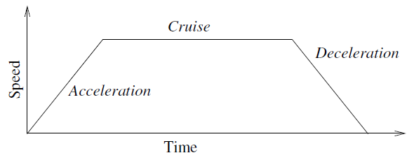
Image source: Universal Robots manual. The diagram shows acceleration, cruise, and deceleration. In this tutorial we use quintic time scaling because it is compact and smooth at the endpoints; part 11 will cover trapezoids, S-curves, and jerk-limited profiles.
What MoveJ actually does
Assume a 6-axis arm:
q_start  = [q1, q2, q3, q4, q5, q6]
q_target = [g1, g2, g3, g4, g5, g6]
MoveJ does not say: "move the TCP in a straight Cartesian line from pose A to pose B." It says: "move each joint from the current angle to the target angle under a common timing law." In other words, we interpolate in joint space:
q(t) = q_start + s(t) * (q_target - q_start)
Here s(t) is a scalar that goes from 0 to 1. When s = 0, the robot is at q_start. When s = 1, the robot is at q_target. If every joint uses the same s(t), all joints arrive exactly at the same final time.
The scalar s(t) should not simply be t / T. Linear interpolation in time creates an instantaneous velocity jump at the start and another jump at the end. A real drive will not like that. Tracking error increases, mechanical vibration appears, and a stiff low-level controller may make the motion feel harsh.
A clean beginner-friendly choice is a quintic polynomial:
u = t / T, 0 <= u <= 1
s(u)  = 10u^3 - 15u^4 + 6u^5
sd(u) = 30u^2 - 60u^3 + 30u^4
sdd(u)= 60u - 180u^2 + 120u^3
This function has zero velocity and zero acceleration at both endpoints. Robotics Toolbox for Python documents jtraj(q0, qf, t) as a joint-space trajectory that uses a fifth-order quintic polynomial with default zero boundary conditions for velocity and acceleration. Our Python prototype below follows the same idea, but keeps the implementation visible so you understand exactly what is happening.
The shortest path in joint space
For a revolute joint, the same physical angle can be represented in multiple ways. For example, 179 deg and -181 deg describe the same direction. If the robot starts at 170 deg and the target is -170 deg, the raw difference is -340 deg, but the shorter physical move is +20 deg.
For a basic MoveJ implementation, continuous revolute joints should use:
delta = wrap_to_pi(q_target - q_start)
wrap_to_pi maps the angle difference into [-pi, pi]. This is what most beginners mean when they say MoveJ should take the shortest joint-space route. On real industrial hardware, the final decision also depends on joint limits, cable routing, hard stops, and whether the axis supports multi-turn motion. A practical controller should let the robot model declare each joint as either continuous or bounded:
if joint is continuous:
    delta = shortest_angular_distance(q_start, q_target)
else:
    delta = q_target - q_start
    check q_target inside [q_min, q_max]
That small distinction prevents many painful bugs. A wrist joint may be safe to wrap. A shoulder joint with a hard stop may not be.
Synchronizing all joints
Suppose joint 1 needs to move 10 degrees, joint 2 needs to move 90 degrees, and joint 3 needs to move 5 degrees. We do not want joint 3 to finish early and wait. A MoveJ command synchronizes the axes with a common duration. The joint that needs the longest time is the bottleneck or leading axis. The other joints use the same duration and therefore move more slowly.
With quintic time scaling:
q_i(t)  = q0_i + delta_i * s(t)
dq_i(t) = delta_i * sd(u) / T
ddq_i(t)= delta_i * sdd(u) / T^2
The maximum of sd(u) is 1.875. The maximum absolute value of sdd(u) is approximately 5.7735. Therefore, for each joint:
T >= abs(delta_i) * 1.875 / v_limit_i
T >= sqrt(abs(delta_i) * 5.7735 / a_limit_i)
Compute both constraints for every joint, then take the maximum over all joints. That maximum is the shared duration T. If the user passes a single v and a like movej(q, a=1.4, v=1.05), you can apply the same limit to all axes for a simple prototype. A production controller should read per-joint limits from the robot model. MoveIt uses URDF or joint_limits.yaml to time-parameterize trajectories according to joint velocity and acceleration limits.
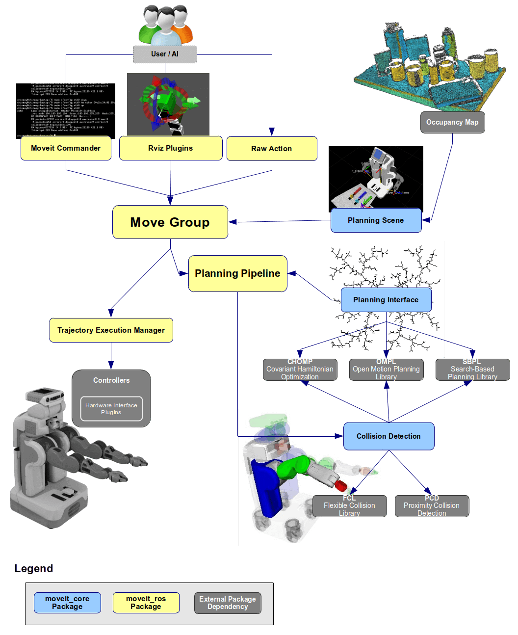
Image source: MoveIt documentation. The MoveJ function in this tutorial is a small, explicit version of the trajectory generation and time parameterization layer: we already have a joint-space path and need to assign valid timing.
Python prototype: jtraj-style quintic
Create movej_quintic.py in any scratch directory:
import numpy as np
import matplotlib.pyplot as plt

def wrap_to_pi(x):
    return (x + np.pi) % (2.0 * np.pi) - np.pi

def quintic_time_scaling(t, T):
    u = np.clip(t / T, 0.0, 1.0)
    s = 10*u**3 - 15*u**4 + 6*u**5
    sd = (30*u**2 - 60*u**3 + 30*u**4) / T
    sdd = (60*u - 180*u**2 + 120*u**3) / (T*T)
    return s, sd, sdd

def compute_duration(delta, v_limit, a_limit):
    delta = np.abs(delta)
    t_vel = np.max(delta * 1.875 / v_limit)
    t_acc = np.max(np.sqrt(delta * 5.7735 / a_limit))
    return max(float(t_vel), float(t_acc), 0.1)

def movej(q_start, q_target, v_limit=1.2, a_limit=2.5, dt=0.01, continuous=True):
    q_start = np.asarray(q_start, dtype=float)
    q_target = np.asarray(q_target, dtype=float)

    if continuous:
        delta = wrap_to_pi(q_target - q_start)
    else:
        delta = q_target - q_start

    v = np.full_like(q_start, v_limit, dtype=float)
    a = np.full_like(q_start, a_limit, dtype=float)
    T = compute_duration(delta, v, a)

    time = np.arange(0.0, T + dt, dt)
    q = []
    qd = []
    qdd = []
    for t in time:
        s, sd, sdd = quintic_time_scaling(t, T)
        q.append(q_start + delta * s)
        qd.append(delta * sd)
        qdd.append(delta * sdd)

    return time, np.array(q), np.array(qd), np.array(qdd), T

if __name__ == "__main__":
    q0 = np.deg2rad([0, -60, 80, 0, 45, 10])
    q1 = np.deg2rad([90, -20, 30, -80, 10, 170])

    t, q, qd, qdd, T = movej(q0, q1, v_limit=1.0, a_limit=2.0, dt=0.01)
    print(f"Move duration: {T:.3f} s")
    print(f"Max speed per joint deg/s: {np.rad2deg(np.max(np.abs(qd), axis=0))}")
    print(f"Max accel per joint deg/s^2: {np.rad2deg(np.max(np.abs(qdd), axis=0))}")

    names = [f"J{i+1}" for i in range(q.shape[1])]
    fig, axes = plt.subplots(2, 1, figsize=(11, 7), sharex=True)

    for i, name in enumerate(names):
        axes[0].plot(t, np.rad2deg(q[:, i]), label=name)
        axes[1].plot(t, np.rad2deg(qd[:, i]), label=name)

    axes[0].set_ylabel("Position (deg)")
    axes[0].set_title("MoveJ joint positions - quintic time scaling")
    axes[0].grid(True)
    axes[0].legend(ncol=3)

    axes[1].set_ylabel("Velocity (deg/s)")
    axes[1].set_xlabel("Time (s)")
    axes[1].set_title("MoveJ joint velocities")
    axes[1].grid(True)
    axes[1].legend(ncol=3)

    plt.tight_layout()
    plt.show()
Run it:
python3 movej_quintic.py
You should see position curves that start and end flat, and velocity curves with smooth bell-like shapes. The joint with the largest effective displacement will usually have the largest velocity. The other joints use the same duration T, so they naturally move more slowly and still arrive at the same time.
This prototype does not check collision, self-collision, fixtures, or forbidden zones. It only proves that the joint-space trajectory is smooth and stays within the kinematic limits we supplied. If you need obstacle-aware motion, continue to the motion planning post later in the series. If you want the taxonomy of point-to-point, linear, spline, and time-parameterized trajectories, read the trajectory types post.
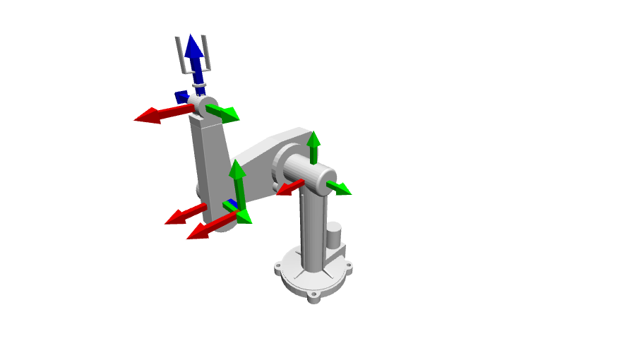
Image source: Robotics Toolbox for Python documentation. The toolbox is useful for checking jtraj, forward kinematics, and the shape of a motion before you port the core idea into a small C++ controller.
Designing a C++ MoveJ API
We want a tiny API that does not depend on ROS:
Trajectory moveJ(q_current, q_target, v_limit, a_limit, dt);
The output should be a vector of setpoints:
time, q[0..N-1], qd[0..N-1], qdd[0..N-1]
In a real servo loop, each control cycle takes the next setpoint and sends it to the joint driver. In a small simulation, we can write the setpoints to CSV and plot them.
Create this folder:
movej_demo/
  CMakeLists.txt
  src/
    main.cpp
CMakeLists.txt:
cmake_minimum_required(VERSION 3.16)
project(movej_demo LANGUAGES CXX)

set(CMAKE_CXX_STANDARD 17)
set(CMAKE_CXX_STANDARD_REQUIRED ON)

add_executable(movej_demo src/main.cpp)
target_compile_options(movej_demo PRIVATE -Wall -Wextra -Wpedantic)
src/main.cpp:
#include <algorithm>
#include <array>
#include <cmath>
#include <fstream>
#include <iomanip>
#include <iostream>
#include <stdexcept>
#include <vector>

constexpr std::size_t DOF = 6;
constexpr double kPi = 3.14159265358979323846;
using Vec = std::array<double, DOF>;

struct Setpoint {
  double t{};
  Vec q{};
  Vec qd{};
  Vec qdd{};
};

struct Trajectory {
  double duration{};
  std::vector<Setpoint> points;
};

double wrapToPi(double x) {
  while (x > kPi) x -= 2.0 * kPi;
  while (x < -kPi) x += 2.0 * kPi;
  return x;
}

Vec subtractTarget(const Vec& q0, const Vec& q1, bool continuous) {
  Vec delta{};
  for (std::size_t i = 0; i < DOF; ++i) {
    const double raw = q1[i] - q0[i];
    delta[i] = continuous ? wrapToPi(raw) : raw;
  }
  return delta;
}

double computeDuration(const Vec& delta, const Vec& v_limit, const Vec& a_limit) {
  double T = 0.1;
  for (std::size_t i = 0; i < DOF; ++i) {
    if (v_limit[i] <= 0.0 || a_limit[i] <= 0.0) {
      throw std::runtime_error("Velocity and acceleration limits must be positive");
    }
    const double d = std::abs(delta[i]);
    const double t_vel = d * 1.875 / v_limit[i];
    const double t_acc = std::sqrt(d * 5.7735 / a_limit[i]);
    T = std::max(T, std::max(t_vel, t_acc));
  }
  return T;
}

void quintic(double t, double T, double& s, double& sd, double& sdd) {
  const double u = std::clamp(t / T, 0.0, 1.0);
  const double u2 = u * u;
  const double u3 = u2 * u;
  const double u4 = u3 * u;
  const double u5 = u4 * u;

  s = 10.0 * u3 - 15.0 * u4 + 6.0 * u5;
  sd = (30.0 * u2 - 60.0 * u3 + 30.0 * u4) / T;
  sdd = (60.0 * u - 180.0 * u2 + 120.0 * u3) / (T * T);
}

Trajectory moveJ(const Vec& q0, const Vec& q_target, const Vec& v_limit,
                 const Vec& a_limit, double dt, bool continuous = true) {
  if (dt <= 0.0) {
    throw std::runtime_error("dt must be positive");
  }

  const Vec delta = subtractTarget(q0, q_target, continuous);
  const double T = computeDuration(delta, v_limit, a_limit);

  Trajectory traj;
  traj.duration = T;

  for (double t = 0.0; t < T + 0.5 * dt; t += dt) {
    const double tc = std::min(t, T);
    double s = 0.0, sd = 0.0, sdd = 0.0;
    quintic(tc, T, s, sd, sdd);

    Setpoint p;
    p.t = tc;
    for (std::size_t i = 0; i < DOF; ++i) {
      p.q[i] = q0[i] + delta[i] * s;
      p.qd[i] = delta[i] * sd;
      p.qdd[i] = delta[i] * sdd;
    }
    traj.points.push_back(p);
  }

  return traj;
}

void writeCsv(const Trajectory& traj, const std::string& path) {
  std::ofstream out(path);
  out << "t";
  for (std::size_t i = 0; i < DOF; ++i) out << ",q" << i + 1;
  for (std::size_t i = 0; i < DOF; ++i) out << ",qd" << i + 1;
  for (std::size_t i = 0; i < DOF; ++i) out << ",qdd" << i + 1;
  out << "\n";

  out << std::fixed << std::setprecision(8);
  for (const auto& p : traj.points) {
    out << p.t;
    for (double x : p.q) out << "," << x;
    for (double x : p.qd) out << "," << x;
    for (double x : p.qdd) out << "," << x;
    out << "\n";
  }
}

int main() {
  const Vec q0 = {0.0, -1.0472, 1.3963, 0.0, 0.7854, 0.1745};
  const Vec q1 = {1.5708, -0.3491, 0.5236, -1.3963, 0.1745, 2.9671};
  const Vec v = {1.0, 1.0, 1.0, 1.0, 1.0, 1.0};
  const Vec a = {2.0, 2.0, 2.0, 2.0, 2.0, 2.0};

  const double dt = 0.008;  // 125 Hz command stream
  const auto traj = moveJ(q0, q1, v, a, dt, true);
  writeCsv(traj, "movej.csv");

  std::cout << "Generated " << traj.points.size() << " setpoints\n";
  std::cout << "Duration: " << traj.duration << " s\n";
  std::cout << "CSV: movej.csv\n";
  return 0;
}
Build and run:
mkdir -p build
cd build
cmake ..
cmake --build .
./movej_demo
The program writes movej.csv. Each row is one timed setpoint. In a real robot controller, you would replace the CSV writer with a driver call. If your hardware accepts position commands only, stream p.q. If it accepts velocity and acceleration feedforward, send p.q, p.qd, and p.qdd.
Minimal playback simulation
Create playback.py next to movej.csv:
import numpy as np
import matplotlib.pyplot as plt
from matplotlib.animation import FuncAnimation

data = np.genfromtxt("movej.csv", delimiter=",", names=True)
t = data["t"]
q = np.vstack([data[f"q{i}"] for i in range(1, 7)]).T

fig, ax = plt.subplots(figsize=(8, 4))
bars = ax.bar([f"J{i}" for i in range(1, 7)], np.rad2deg(q[0]))
ax.set_ylim(-190, 190)
ax.set_ylabel("Joint position (deg)")
ax.set_title("MoveJ playback from C++ CSV")
time_text = ax.text(0.02, 0.92, "", transform=ax.transAxes)

def update(frame):
    for bar, value in zip(bars, np.rad2deg(q[frame])):
        bar.set_height(value)
    time_text.set_text(f"t = {t[frame]:.3f} s")
    return list(bars) + [time_text]

ani = FuncAnimation(fig, update, frames=len(t), interval=8, blit=True)
plt.show()
Run:
python3 playback.py
This is not a 3D kinematic simulator yet, but it verifies the important part of MoveJ: setpoints are sampled at a fixed period, all joints arrive at the same final time, and the motion is smooth. To connect it to a real simulator, replace the bar chart with FK and a viewer. Robotics Toolbox, PyBullet, MuJoCo, or your own WebGL viewer can all consume the same q(t) stream.
Safety checklist for your first MoveJ
Before sending MoveJ to real hardware, check these items:
| Check | Why it matters |
|---|---|
q_target is inside joint limits |
Avoid impossible commands |
| Wrapping is correct per joint | Avoid unexpected long rotations |
max(abs(qd)) <= v_limit |
Protect drives and gearboxes |
max(abs(qdd)) <= a_limit |
Reduce vibration and tracking error |
| Setpoint period matches the servo loop | Avoid timing jitter |
| Start state comes from live feedback | Avoid a jump at the first sample |
| Stop conditions exist | Stop on tracking error, E-stop, or protective stop |
One common beginner mistake is using an old internal q_start instead of the latest encoder feedback. If an operator jogged the robot, gravity compensation moved slightly, or the controller restarted, the first setpoint can jump. Always seed MoveJ from fresh robot feedback.
MoveJ versus MoveL
This article focuses on MoveJ, but the contrast with MoveL matters:
| Command | Interpolation | Strength | Weakness |
|---|---|---|---|
| MoveJ | Joint space | Fast, stable, easy to limit per joint | TCP path is curved and hard to predict |
| MoveL | Cartesian space | TCP follows a straight line | Needs continuous IK and may hit singularities |
Use MoveJ for free moves: home to approach, one safe region to another, or fast repositioning where the exact TCP path is not important. Use MoveL when the tool itself must follow a line, such as a gripper moving straight down to pick an object. A common pick-and-place pattern is MoveJ to an approach point, MoveL down, MoveL back up, and MoveJ to the next region.
Connection to velocity profiles in part 11
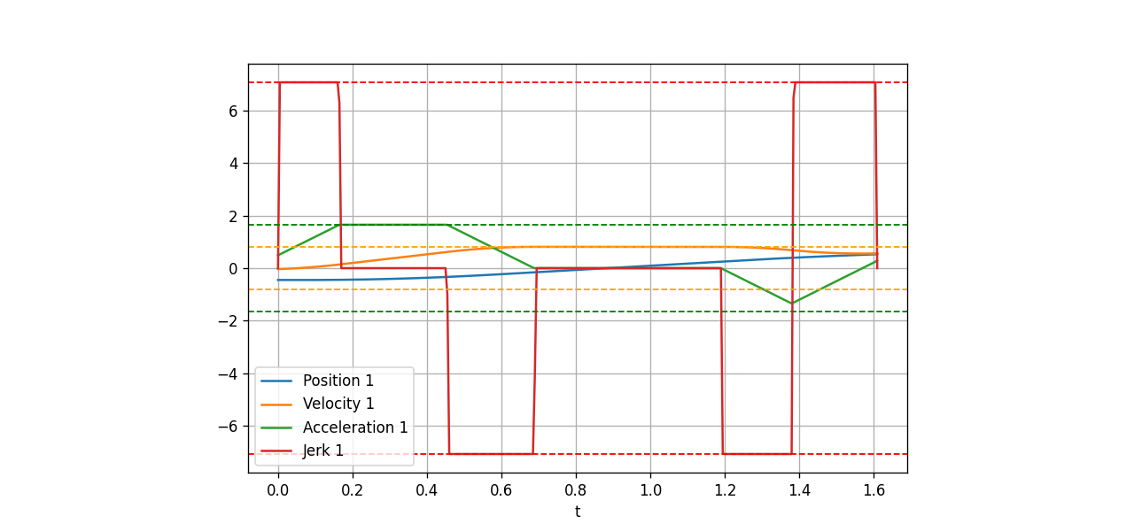
Quintic time scaling is excellent for learning because the formula is short and the endpoints are smooth. It is not the most time-optimal industrial profile. Real controllers often use trapezoidal, S-curve, or jerk-limited profiles. Ruckig, for example, generates trajectories from a current state to a target state under velocity, acceleration, and jerk constraints, and it can run online in a control loop. MoveIt 2 also includes time parameterization and can apply Ruckig smoothing to reduce jerk after planning.
In part 11 on velocity profiles, we will replace the quintic() function with trapezoidal, S-curve, and jerk-limited profiles. The architecture stays the same:
q_start, q_target
  -> per-joint delta
  -> choose shared duration/profile
  -> sample q, qd, qdd at dt
  -> stream setpoints to the servo loop
When a controller needs jerk limits and online reaction, a dedicated trajectory generation library can replace the handwritten time law. The featured image of this post uses a trajectory plot from Ruckig to highlight that bridge between basic MoveJ and advanced velocity profiles.
References
- Universal Robots Script Manual: movej(q, a, v, t, r)
- Universal Robots PolyScope Move command documentation
- Robotics Toolbox for Python: trajectories and jtraj
- MoveIt 2 documentation: Time Parameterization
- Ruckig documentation: online trajectory generation tutorial
Conclusion
You now have a minimal but structurally correct MoveJ implementation: choose the shortest joint-space displacement, compute a shared duration from velocity and acceleration limits, use quintic time scaling to generate q, qd, and qdd, build the C++ program with CMake, export CSV, and play the motion back in a tiny simulation.
This is not just a toy. A clean MoveJ is the first brick of a robot arm controller. Once this layer is correct, you can add per-axis joint limits, collision checking, blending, jerk-limited profiles, real robot interfaces, and eventually full motion planning without being confused about timed setpoint generation.