You want to build a real robot arm controller, but the first documents you open immediately throw a dense vocabulary at you: FK, IK, Jacobian, MoveJ, MoveL, MoveC, trajectory generation, interpolation, servo control, driver interfaces, ROS 2 control, MoveIt 2, Ruckig, Pinocchio, KDL. If you start from a large framework, you may run a demo without understanding why the robot moved that way. If you start from equations only, you may understand a few mathematical blocks but still not know how to turn them into smooth commands for real hardware.
This series takes the middle path: classical robot arm control. By classical, I mean a controller built from geometry, kinematics, joint limits, velocity and acceleration constraints, trajectory profiles, interpolation, and feedback loops. This is the foundation behind most industrial arms, whether you work with Universal Robots, ABB, FANUC, KUKA, Franka Panda, or a custom manipulator. It is different from learning-based or VLA-based manipulation because we are not learning a direct mapping from image and language to motor action. We model the robot, plan a valid motion, generate a time-parameterized trajectory, then send setpoints to the servo loop at a fixed control period.
That does not make learning or VLA irrelevant. Models like the ones discussed in VLA models for robotics are powerful when the robot needs perception, language grounding, demonstrations, or data-driven policies. But once a high-level policy says "move the tool to this pose" or "follow this line", a classical controller still has to produce safe joint commands. In a practical stack, a VLA can be the task-level brain, while the classical controller is the motion system that keeps the robot inside limits.
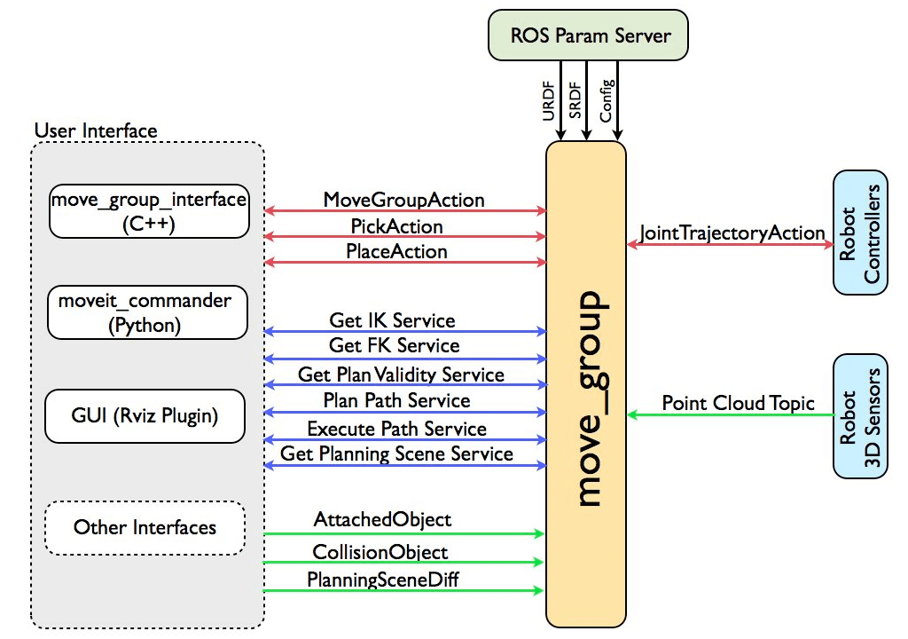
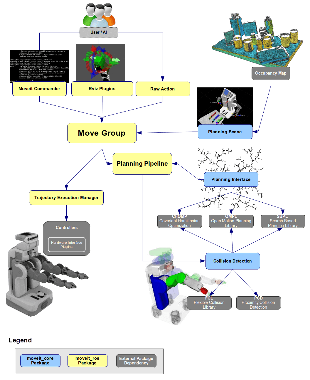
Image source: MoveIt documentation. The diagram shows user interfaces, planning scene, controllers, and robot sensors connected through an integration node such as move_group.
Roadmap series
This is part 1 of 15 in the series Classical Robot Arm Controller (C++ & Python): From FK/IK to MoveJ, MoveL, Jogging and Motion Planning. Read the posts in this order:
- robot-arm-classical-controller-1-roadmap - Controller stack, learning philosophy, tool choices, and the 2026 library map.
- robot-arm-classical-controller-2-cpp-cmake-setup - C++17/20, CMake, Eigen, unit tests, and a clean controller project structure.
- robot-arm-classical-controller-3-robot-model - Robot model, URDF, joint limits, frame trees, link transforms, and model data structures.
- robot-arm-classical-controller-4-forward-kinematics - Forward kinematics, inverse kinematics, Jacobians, singularities, and Python validation.
- robot-arm-classical-controller-5-inverse-kinematics - Numerical IK: damped least squares, task priorities, limit handling, Pinocchio, pink, and mink.
- robot-arm-classical-controller-6-jacobian - Advanced topics: redundancy, null-space control, force-aware planning, and multiple simultaneous constraints.
- robot-arm-classical-controller-7-frames - Base frames, tool frames, world frames, and joint or Cartesian jogging.
- robot-arm-classical-controller-8-movej - MoveJ and MoveL: the difference between joint-space and Cartesian-space motion.
- robot-arm-classical-controller-9-movel - Trajectory types: point-to-point, linear, spline, and time-parameterized paths.
- robot-arm-classical-controller-10-movec-movep - MoveC, circular arcs, via points, welding, dispensing, and polishing applications.
- robot-arm-classical-controller-11-profiles - Velocity profiles: trapezoidal, S-curve, jerk-limited profiles, and Ruckig.
- robot-arm-classical-controller-12-blending - Waypoint blending, corner radius, and the tradeoff between accuracy and cycle time.
- robot-arm-classical-controller-13-jogging-servo - Online jogging servo loops, singularity scaling, and collision stop logic.
- robot-arm-classical-controller-14-motion-planning - Obstacle-aware motion planning: sampling, collision checking, MoveIt 2, and cuRobo.
- robot-arm-classical-controller-15-ros2-ur-rtde - End-to-end integration: simulation first, UR5/Panda models,
ur_rtde, logging, and safety.
Classical control versus learning and VLA
A classical controller starts from an explicit model. We know how many joints the robot has, the position and velocity limits of each joint, the length and transform of each link, the location of the tool frame, and the relationship between base, world, and sensor frames. When a user calls MoveL(pose), the controller does not guess a motor action with a neural network. It solves a chain of deterministic problems:
- Is the target pose inside the reachable workspace?
- Is there a valid IK solution?
- Is the Cartesian line collision-free?
- When the path is converted into a time trajectory, which joint reaches its velocity or acceleration limit first?
- What setpoint should be sent at a 1 ms, 2 ms, or 8 ms control period?
- If the real robot reports tracking error, protective stop, network delay, or emergency stop, how should the controller react?
Learning-based manipulation starts from data. The OpenVLA paper, for example, describes a vision-language-action policy trained from large-scale robot demonstrations and vision-language data, then fine-tuned for downstream robot tasks. This is useful for perception-heavy manipulation and language-conditioned behavior. However, it does not remove the need for a hard safety layer underneath. A learned policy may choose a target pose, a grasp, or a subtask. The classical controller still has to keep the motion inside joint limits, avoid obstacles, respect servo bandwidth, and stop safely when the physical world disagrees with the plan.
In practice, robotics engineers should understand both sides. If you work on AI robotics, classical control lets you debug actions, evaluate safety, and connect policies to hardware. If you work on industrial automation, learning helps you add perception and adaptation. This series focuses on the classical layer because it is the layer that must work before a real arm moves at production speed.
Controller stack: from user command to motor current
A robot arm controller is not a single move_to(target) function. It is a stack of layers, where each layer turns a broad intent into a more concrete command:
User command
  MoveJ(q_goal), MoveL(T_goal), MoveC(T_mid, T_goal), Jog(v)
        |
        v
Motion planner
  feasibility, IK search, collision check, path constraints
        |
        v
Trajectory generator
  path -> time law, velocity/acceleration/jerk limits
        |
        v
Interpolator
  sample trajectory at control period: q, dq, ddq
        |
        v
Servo loop
  feedback control, tracking error, safety checks
        |
        v
Joint driver
  position/velocity/torque command to hardware
        |
        v
Robot arm
  encoders, current, force/torque, status feedback
The same idea as a Mermaid diagram:
flowchart TD
  A[User API: MoveJ / MoveL / MoveC / Jog] --> B[Command validator]
  B --> C[Motion planner]
  C --> D[Trajectory generator]
  D --> E[Interpolator at control cycle]
  E --> F[Servo loop]
  F --> G[Joint driver]
  G --> H[Robot arm hardware]
  H --> I[State feedback: joint state, IO, FT, safety]
  I --> F
  I --> C
1. User command: MoveJ, MoveL, MoveC, Jog
This is the API used by an operator program or by a higher-level robot application. MoveJ usually means moving from the current joint vector to a target joint vector through a smooth path in joint space. The tool may trace a curved line in Cartesian space, but the joint motion is simple and stable. MoveL means the tool center point follows a straight line in Cartesian space. The controller must solve IK along the path, because every point on the line needs a valid joint configuration. MoveC follows a circular arc through a via point and is common in welding, dispensing, and polishing. Jog is continuous low-speed control: hold +X and the tool moves along an axis in the base or tool frame.
A beginner mistake is to think MoveJ and MoveL are just two names for the same move. They are different because they constrain different spaces. MoveJ prioritizes smooth joint motion. MoveL prioritizes the geometric path of the tool.
2. Motion planner: finding a valid path
The motion planner answers: "Is there a path from state A to state B that avoids collisions and satisfies constraints?" In a simple empty scene, the planner might only check IK and joint limits. In a real workcell with a table, fixtures, gripper geometry, cameras, and safety zones, it must reason about a planning scene and collision geometry. MoveIt 2 describes itself as the robotic manipulation platform for ROS 2, covering motion planning, manipulation, 3D perception, kinematics, and control. In this series, we will not start by hiding everything inside MoveIt. We will build small versions first, then use MoveIt 2 later so the framework is no longer a black box.
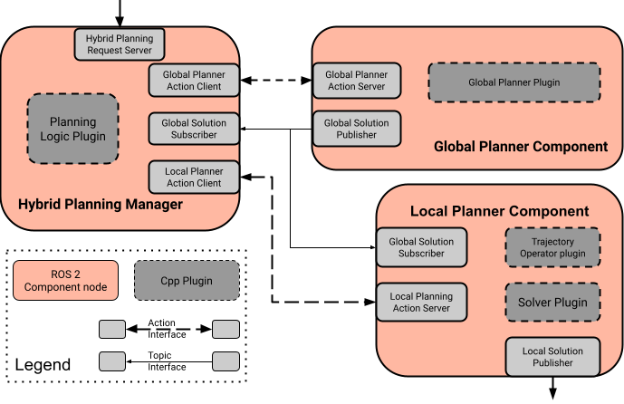
Image source: MoveIt 2 documentation. Hybrid planning separates a global planner from a local planner, allowing a robot to combine long-horizon planning with online reaction.
3. Trajectory generator: adding time to a path
A path tells the robot where to go. A trajectory tells the robot when to be at each point, and with what velocity and acceleration. This is where velocity, acceleration, and jerk limits matter. If you simply interpolate position linearly with time, the robot can jerk at the start and end of the motion. A trapezoidal velocity profile is better, but acceleration still changes abruptly. An S-curve or jerk-limited profile produces smoother motion and less vibration.
Ruckig is a key library at this layer. Its documentation describes online trajectory generation from a current state to a target state under velocity, acceleration, and jerk limits. This is exactly the kind of component a practical controller needs: at every cycle it can update the state and generate the next setpoint.
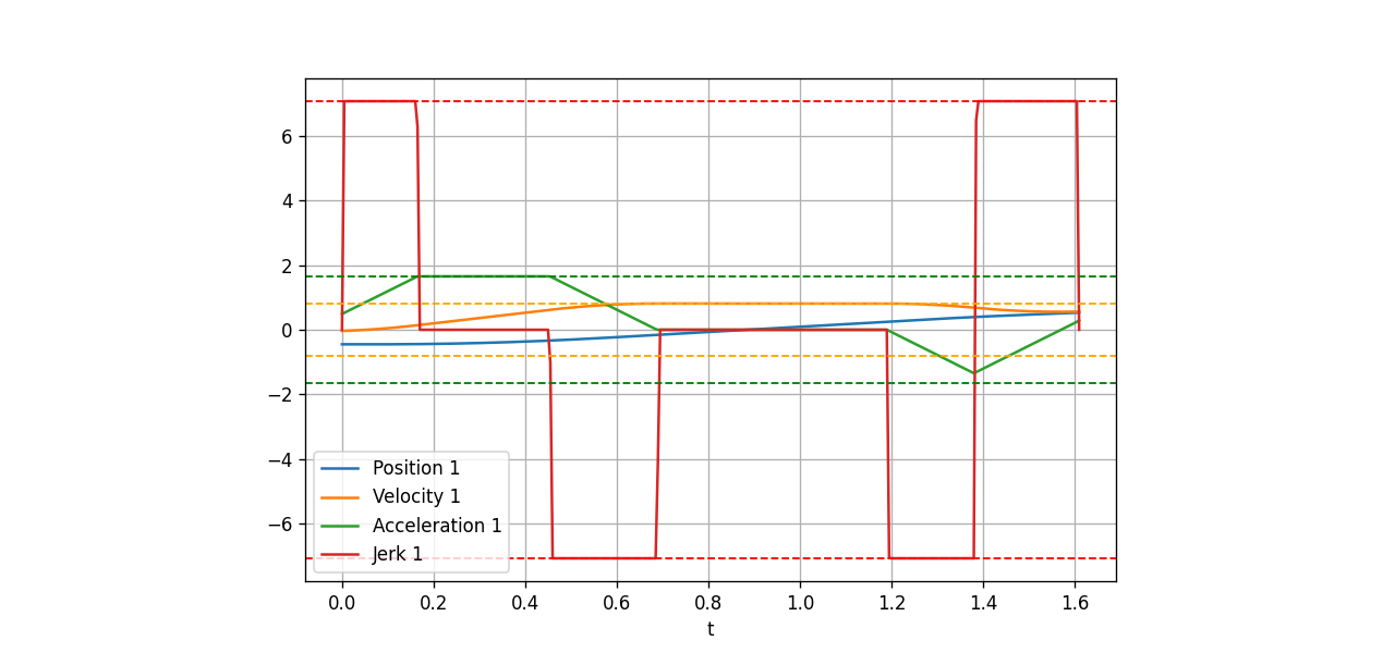
Image source: Ruckig documentation. A real trajectory is not only position. It also includes velocity, acceleration, and jerk.
4. Interpolator: sampling at the control period
A servo loop does not consume an abstract path. It needs setpoints at each tick: q_des(t), dq_des(t), sometimes ddq_des(t) or torque feedforward. If the controller runs at 500 Hz, the interpolator must produce a new point every 2 ms. If it runs at 125 Hz, it produces a point every 8 ms. This layer is sensitive to timing. Scheduler delay, network jitter, clock drift, and missed cycles can all cause visible motion artifacts.
5. Servo loop: feedback and safety
The servo loop is where desired motion meets physical state. If encoders report that a joint is lagging, the controller reacts within allowed limits. If tracking error exceeds a threshold, it stops. If force/torque feedback suggests contact, it slows down or triggers a protective stop. If the robot is jogging near a singularity, it scales velocity to prevent joint speeds from exploding. This is why real controllers are usually written in C++: deterministic behavior, low allocation, predictable latency, native drivers, ROS 2 integration, and Eigen-based math.
6. Joint driver: talking to hardware
The driver sends commands to the robot: position, velocity, or torque. For Universal Robots, ur_rtde provides a C++ interface and Python bindings for control and state feedback through RTDE. In ROS 2, the driver often connects through ros2_control and FollowJointTrajectory. On closed industrial controllers, you may have only a vendor API. The interface differs, but the principle is the same: do not send commands beyond limits, do not assume the network is perfect, and always define a safe stop strategy.
Teaching philosophy: three layers for every mathematical idea
Every major concept in this series will be taught in three layers. We will not jump directly into a library.
Layer 1: calculate by hand to understand the idea. For FK, we multiply the transform matrices of a two-link or three-link arm. For the Jacobian, we compute each column from a joint axis and the vector to the end-effector. For IK, we solve a planar two-link robot before talking about six-degree-of-freedom arms. The goal is not to do math for its own sake. The goal is to understand signs, frames, radians versus degrees, and the physical reason singularities appear.
Layer 2: code from scratch. Once the equation is clear, we write a minimal version in C++ or Python: joint vectors, homogeneous transforms, an FK function, damped least-squares IK, trapezoidal trajectories, and a small S-curve implementation. This code is not meant to replace production libraries. It is a microscope. When MoveIt, Pinocchio, or a vendor driver produces a surprising result, your tiny implementation gives you a baseline.
Layer 3: use modern, well-known libraries. After the principle is understood, we use Eigen, Pinocchio, KDL, Ruckig, TOPP-RA, MoveIt 2, pink, mink, cuRobo, and ur_rtde. At that point a library is no longer a black box. You know which problem it solves, what the important inputs are, and how to validate the output.
Tool philosophy: C++ for real controllers, Python for fast validation
This series uses two languages, with different responsibilities.
C++ is the main language for the real controller. We will use CMake for project structure, Eigen for linear algebra, unit tests to lock behavior, and data structures that avoid unnecessary allocation inside servo loops. For code close to hardware, C++ remains a practical choice because of latency, native driver support, ROS 2 ecosystem integration, and control over memory and timing.
Python is the laboratory. NumPy, robotics-toolbox-python, and matplotlib help you prototype FK, IK, and trajectory logic quickly. You can plot joint velocity, inspect singularities, compare multiple IK methods, and validate C++ results numerically. Python is not the hard real-time layer, but it dramatically shortens the algorithm debugging loop.
Simulation first. We will prefer UR5/UR5e and Franka Panda models because they are widely used, easy to find as URDF models, and well supported in tutorials. Run in simulation, log trajectories, check limits, verify frames, then connect to real hardware. If you cannot measure it in simulation, you should not send it to a real robot arm.
For a broader example of simulation-first thinking and telemetry, see G1 MuJoCo telemetry: DDS and simulation-first. It is about humanoids, but the engineering habit of logging, replaying, and validating before touching hardware applies directly to robot arms.
Library ecosystem as of June 2026
The table below summarizes the libraries used in the rest of the series. Versions were checked against GitHub, PyPI, ROS docs, or official documentation on June 13, 2026.
| Library | June 2026 status | What we use it for | Posts in this series |
|---|---|---|---|
| Eigen | Standard C++ linear algebra dependency | Vectors, matrices, transforms, small solvers | Parts 2, 3, 4, 5 |
| Pinocchio | 4.0.0 is latest; 3.9.0 is the final recent 3.x release before breaking changes | FK, Jacobians, dynamics, URDF model loading | Parts 4, 5, 6 |
| robotics-toolbox-python | 1.1.1 on PyPI | Python FK/IK prototyping, plotting, validation | Parts 3, 4, 5 |
| Orocos KDL | Long-standing C++/ROS kinematics library | Chains, FK solvers, IK solvers, PyKDL | Parts 4, 5 |
| Ruckig | Official docs show API 0.19.3; PyPI community package is 0.17.3 | Online jerk-limited trajectory generation | Parts 11, 13 |
| TOPP-RA / toppra | 0.6.8 on PyPI, released May 3, 2026 | Time-optimal path parameterization under constraints | Parts 9, 11, 12 |
| MoveIt 2 | Rolling package 2.14.1; binaries for Humble, Jazzy, Rolling | Planning scene, collision checking, OMPL, execution | Parts 14, 15 |
| pink | pin-pink 4.2.0, released Apr 20, 2026 |
Pinocchio-based differential IK with tasks and limits | Parts 5, 6, 13 |
| mink | 1.1.1, released May 15, 2026 | MuJoCo-based differential IK with tasks, limits, and collision logic | Parts 5, 7, 13 |
| NVIDIA cuRobo | v0.8.0/cuRoboV2 announced in Apr 2026 | GPU IK, collision checking, trajectory optimization, planning | Part 14 |
| ur_rtde | 1.6.3, released Mar 13, 2026 | Control and state feedback for Universal Robots through RTDE | Part 15 |
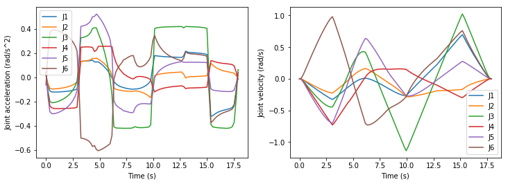
Image source: TOPP-RA documentation. Path parameterization turns a geometric path into a trajectory that satisfies velocity and acceleration constraints.
A simple command through the whole stack
Suppose your application calls:
robot.MoveL(
  Pose::FromXYZRPY(0.45, -0.10, 0.32, 3.14, 0.0, 1.57),
  Speed{0.25},
  Accel{0.8}
);
The controller then works through the stack:
- Validate the target pose in the selected frame.
- Build a Cartesian line from the current pose to the target pose.
- Discretize the line, for example every 2 mm or based on curvature.
- Run IK for each point and choose solutions continuous with the current joint state.
- Check joint limits, velocity limits, singularities, and collisions.
- Time-parameterize the joint path with a suitable velocity profile.
- At each servo cycle, interpolate
q_des,dq_des, and possiblyddq_des. - Send commands to the driver, read feedback, and check error conditions.
- Continue if the error is small. Slow down or stop if the error is unsafe.
If a VLA is in the system, it may decide the target pose or subtask at the beginning. But steps 2 through 9 are still classical control. This is why the series is useful even if your final application includes robot learning.
When to use libraries and when to write code yourself
Writing every component from scratch for production is risky. Using large libraries without understanding them is also risky. A pragmatic rule is:
- Write small versions of FK, Jacobians, planar IK, trapezoidal profiles, and interpolation for learning and tests.
- Use Eigen instead of creating your own matrix library.
- Use Pinocchio or KDL when the robot model becomes complex or you need URDF support.
- Use Ruckig or TOPP-RA when trajectories must respect velocity, acceleration, and jerk limits.
- Use MoveIt 2 when you need a planning scene, collision world, planning plugins, and ROS 2 integration.
- Use cuRobo when you have an NVIDIA GPU and need fast planning over many IK or collision queries.
- Use
ur_rtdeor a vendor driver when you touch real hardware. Do not reverse-engineer a robot protocol unless you have a very good reason.
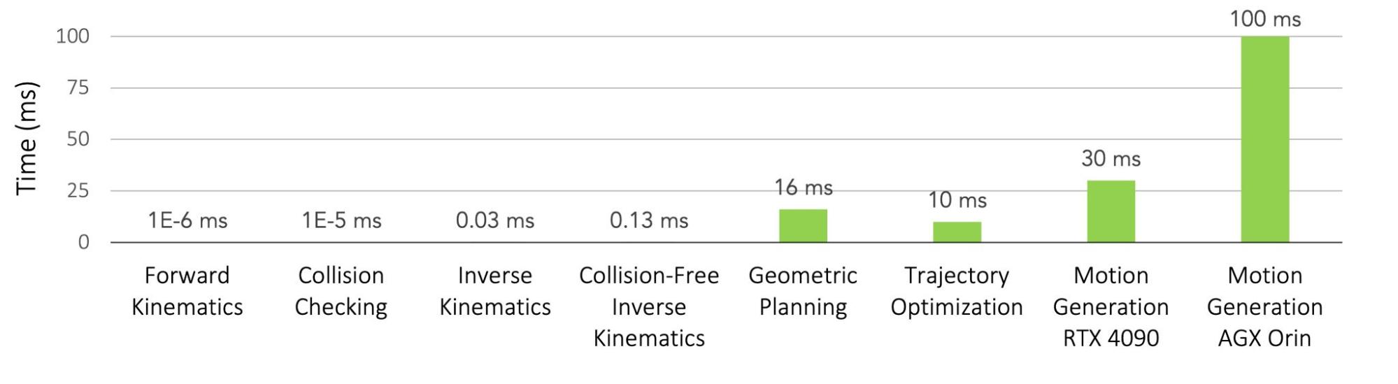
Image source: NVIDIA Technical Blog. GPU motion generation can reduce compute time for IK, collision checking, and multi-seed planning problems.
What you should understand after this post
After this opening article, you should be able to explain the main blocks of an industrial arm controller:
MoveJ,MoveL,MoveC, andJogare user-level commands, not the whole controller.- The motion planner finds a valid path under constraints and collision checks.
- The trajectory generator adds time, velocity, acceleration, and jerk limits to a path.
- The interpolator samples the trajectory at the control period.
- The servo loop uses feedback to track setpoints and handle safety.
- The joint driver communicates with real hardware or a simulator.
- C++ is the right center of gravity for real controllers; Python is the right laboratory for prototyping and validation.
- Simulation-first development reduces risk before UR5/Panda models or real robots are involved.
The next post sets up the C++/CMake/Eigen project foundation before we implement robot models, FK, IK, and trajectories. If you want to peek ahead, read MoveJ and MoveL or the later motion planning entry in the roadmap.
References
- MoveIt 2 documentation and MoveIt concepts
- Ruckig documentation and Ruckig on PyPI
- TOPP-RA documentation and toppra on PyPI
- Pinocchio releases
- OpenVLA paper
- NVIDIA cuRobo documentation and NVIDIA Technical Blog on cuRobo
- ur_rtde on PyPI