In the MoveJ and MoveL article, we separated joint-space moves from Cartesian straight-line moves. In the MoveC and MoveP article, we added circular arcs and process paths. This article focuses on a smaller idea that has a large impact on how industrial robot motion feels: waypoint blending, also called corner smoothing.
Suppose you teach a robot a sequence such as P0 -> P1 -> P2 -> P3. The simplest controller runs one segment at a time: MoveL to P1, stop, MoveL to P2, stop, then continue. That is easy to reason about, but it is slow and often mechanically harsh. In welding, glue dispensing, painting, polishing, camera scanning, or high-speed pick-and-place, stopping at every waypoint can ruin the process: glue accumulates at corners, paint becomes thicker, polishing force spikes, scan velocity becomes inconsistent, and cycle time grows quickly.
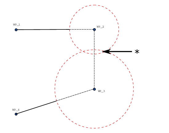
Blending solves this by allowing the TCP to not pass exactly through the nominal waypoint. The robot leaves the incoming segment before the corner, follows a small curved transition, then joins the outgoing segment. The most common parameter is blend radius: the allowed smoothing radius around the waypoint. A larger radius lets the robot keep more speed, but also causes more path deviation. That is the core tradeoff in this article: path accuracy is exchanged for speed and smoothness.
1. Why hard stops at every waypoint are slow
Consider a robot moving along segment P0 -> P1 and then changing direction to P1 -> P2. If the TCP must hit P1 exactly and the two segments are not collinear, the velocity vector before and after the waypoint points in different directions. On real hardware, velocity cannot change direction instantly because acceleration is bounded. If the controller must guarantee that it passes through the sharp corner, the safe solution is to reduce speed to zero at P1, then accelerate again in the new direction.
That creates three costs:
- Time cost: every waypoint adds deceleration and acceleration phases. With 50 waypoints, the time spent ramping can dominate the time spent moving at process speed.
- Mechanical cost: repeated stop-start motion increases force variation in motors, gearboxes, belts, screws, and structural components.
- Process cost: the tool keeps doing work while the TCP slows down or stops. For glue, welding, painting, and grinding, non-uniform speed often means non-uniform quality.
Universal Robots describes blend radius as a way for the robot trajectory to blend around the waypoint so the robot does not stop at that point. The same documentation also notes that blending can make a program run faster because it avoids slowing down and accelerating between trajectories. This is not vendor magic. It is a direct consequence of kinematics: if you want to change direction at nonzero speed, you need finite acceleration over a finite curve.
For a circular transition with radius r and linear speed v, the centripetal acceleration is approximately:
a_c = v^2 / r
If r is small and you still want a high v, the required acceleration grows quickly. Given an acceleration limit a_max, the corner speed must satisfy:
v <= sqrt(a_max * r)
This equation is a useful mental model for choosing a blend radius. A small radius keeps the path close to the waypoint, but forces the robot to slow down. A large radius allows higher speed, but the TCP cuts farther away from the nominal corner. In a process path, r should be chosen from path tolerance, acceleration limits, distance to obstacles, and process quality requirements.
2. What blend radius means
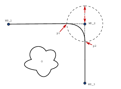
For three consecutive points P0, P1, P2, the waypoint to blend is P1. There are two line segments:
- Incoming segment:
P0 -> P1 - Outgoing segment:
P1 -> P2
If r = 0, the robot has to reach P1. If r > 0, the controller creates a transition curve near P1. A common simple implementation uses a circular arc tangent to both line segments. The tangent condition matters: the velocity direction at the blend entry matches the incoming line, and the velocity direction at the blend exit matches the outgoing line. If scalar speed is also continuous, the velocity vector changes smoothly instead of snapping.
For a simple circular blend:
u = normalize(P1 - P0)      # incoming travel direction
v = normalize(P2 - P1)      # outgoing travel direction
a = -u                      # ray from the corner back toward P0
b = v                       # ray from the corner toward P2
phi = angle(a, b)           # interior angle at the waypoint
d = r / tan(phi / 2)        # trim distance from the waypoint
T_in  = P1 - u * d
T_out = P1 + v * d
T_in is where the robot leaves the incoming line. T_out is where it rejoins the outgoing line. Between them, the robot follows a circular arc of radius r. The new path is:
P0 -> ... -> T_in -> arc(T_in, T_out) -> T_out -> ... -> P2
The robot does not touch P1. The maximum deviation is localized around the corner. In many industrial APIs, blend radius means a zone in which the robot is allowed to smooth around the waypoint, not necessarily a formal promise that every point on the arc is exactly r away from the waypoint. If you build your own controller, define this precisely: is r the mathematical arc radius, or is it the allowed waypoint zone radius?
3. When blending is invalid
Blending cannot always be applied. A beginner-friendly controller should check at least three conditions.
First, neighboring segments must be long enough. With the formula above, the trim distance d must not exceed the length of the incoming or outgoing segment. If P0-P1 is too short, there is not enough room to leave the straight segment before the corner. A conservative rule is d < 0.5 * min(len_in, len_out) when many waypoints are close together.
Second, consecutive blends must not overlap. Universal Robots explicitly documents that blends cannot overlap; if the radius around one waypoint overlaps the radius around a previous or following waypoint, the program should warn or reduce the radius. Your own controller should do the same. Before moving real hardware, compute T_in/T_out for the whole waypoint chain and verify that the intervals along each segment are still ordered.
Third, a valid TCP path does not guarantee a valid robot trajectory. Cartesian blending only describes the end-effector path. After that, you still need inverse kinematics, joint limit checks, singularity checks, collision checks, and velocity/acceleration/jerk limits per joint. Near a singularity, a gentle TCP arc can require very high joint speed. A robust pipeline usually looks like this:
Cartesian waypoints
-> build blended geometric path
-> sample by arc length
-> solve continuous IK using the previous sample as seed
-> time-parameterize with joint limits
-> verify TCP error, collision, and limits again
MoveIt/Pilz also separates Cartesian limits for LIN/CIRC commands from the final joint trajectory. Its output is a joint trajectory with positions, velocities, accelerations, and timestamps. If planning fails because of joint-space limits, the user needs to reduce scaling or modify the path. The lesson is simple: do not send a nice-looking 2D TCP plot directly to servo control without joint-space verification.
4. Python prototype: circular corner blend and velocity continuity
The prototype below uses only numpy and matplotlib. It takes a 2D polyline, replaces each corner with a tangent circular arc, samples the resulting path by distance, and estimates velocity so you can inspect continuity. It is written in 2D for clarity. The same idea extends to 3D by constructing a local blend plane for each corner.
import numpy as np
import matplotlib.pyplot as plt

EPS = 1e-9

def normalize(x):
    n = np.linalg.norm(x)
    if n < EPS:
        raise ValueError("Vector is too small")
    return x / n

def angle_between(a, b):
    c = np.clip(np.dot(a, b), -1.0, 1.0)
    return np.arccos(c)

def rot90(x):
    return np.array([-x[1], x[0]])

def line_intersection(p, dp, q, dq):
    # p + s*dp = q + t*dq
    A = np.column_stack([dp, -dq])
    rhs = q - p
    if abs(np.linalg.det(A)) < 1e-9:
        raise ValueError("Lines are nearly parallel")
    s, _ = np.linalg.solve(A, rhs)
    return p + s * dp

def blend_corner(p0, p1, p2, radius, ds=0.005):
    p0, p1, p2 = map(lambda p: np.asarray(p, dtype=float), [p0, p1, p2])
    u = normalize(p1 - p0)
    v = normalize(p2 - p1)

    # Interior angle between the ray back to p0 and the ray toward p2.
    a = -u
    b = v
    phi = angle_between(a, b)
    if phi < np.deg2rad(5) or abs(np.pi - phi) < np.deg2rad(1):
        return None

    d = radius / np.tan(phi / 2.0)
    len_in = np.linalg.norm(p1 - p0)
    len_out = np.linalg.norm(p2 - p1)
    if d > 0.45 * min(len_in, len_out):
        raise ValueError(f"Blend radius is too large: trim distance {d:.3f} m")

    t_in = p1 - u * d
    t_out = p1 + v * d

    # The circle center is the intersection of two normals at the tangent points.
    n1 = rot90(u)
    n2 = rot90(v)
    candidates = [
        line_intersection(t_in, n1, t_out, n2),
        line_intersection(t_in, -n1, t_out, n2),
    ]
    center = min(candidates, key=lambda c: abs(np.linalg.norm(c - t_in) - radius))

    def theta(p):
        r = p - center
        return np.arctan2(r[1], r[0])

    th0 = theta(t_in)
    th1 = theta(t_out)

    def sample(th_start, th_end):
        arc_len = abs(th_end - th_start) * radius
        n = max(3, int(np.ceil(arc_len / ds)) + 1)
        th = np.linspace(th_start, th_end, n)
        pts = center + radius * np.column_stack([np.cos(th), np.sin(th)])
        return pts

    options = [
        sample(th0, th1),
        sample(th0, th1 + 2 * np.pi),
        sample(th0, th1 - 2 * np.pi),
    ]

    def tangent_error(pts):
        tan0 = normalize(pts[1] - pts[0])
        tan1 = normalize(pts[-1] - pts[-2])
        return np.linalg.norm(tan0 - u) + np.linalg.norm(tan1 - v)

    arc = min(options, key=tangent_error)
    return t_in, t_out, center, arc

def blended_path(points, radius, ds=0.005):
    points = [np.asarray(p, dtype=float) for p in points]
    out = [points[0]]

    for i in range(1, len(points) - 1):
        p0, p1, p2 = points[i - 1], points[i], points[i + 1]
        blend = blend_corner(p0, p1, p2, radius, ds)
        if blend is None:
            out.append(p1)
            continue
        t_in, t_out, center, arc = blend
        out.append(t_in)
        out.extend(arc[1:-1])
        out.append(t_out)

    out.append(points[-1])
    return np.array(out)

def finite_difference_velocity(path, dt):
    return np.diff(path, axis=0) / dt

polyline = np.array([
    [0.00, 0.00],
    [0.45, 0.00],
    [0.65, 0.25],
    [0.95, 0.25],
    [1.05, -0.10],
])

path = blended_path(polyline, radius=0.08, ds=0.004)
dt = 0.01
vel = finite_difference_velocity(path, dt)
speed = np.linalg.norm(vel, axis=1)

fig, (ax0, ax1) = plt.subplots(1, 2, figsize=(12, 4))
ax0.plot(polyline[:, 0], polyline[:, 1], "o--", label="original waypoints")
ax0.plot(path[:, 0], path[:, 1], "-", label="blended path")
ax0.axis("equal")
ax0.grid(True)
ax0.legend()

ax1.plot(speed)
ax1.set_title("Approximate speed after uniform sampling")
ax1.set_xlabel("sample")
ax1.set_ylabel("|v|")
ax1.grid(True)
plt.tight_layout()
plt.show()
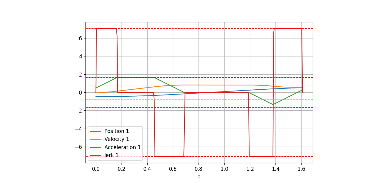
The important thing to inspect is not whether the plot looks pretty, but whether the path has tangent continuity. At T_in, the arc is tangent to the incoming line. At T_out, the arc is tangent to the outgoing line. If scalar speed is continuous, the velocity vector is continuous in direction as well. Acceleration, however, still has a discontinuity because curvature changes from 0 on the straight line to 1/r on the circular arc. For even smoother motion, use clothoids, splines, or jerk-limited time parameterization. For a classical controller, circular blends plus a jerk-limited profile are already a major improvement over hard stops at every waypoint.
5. Choosing radius from speed, tolerance, and obstacles
A practical estimate is:
r_min = v_process^2 / a_allowed
If the process requires a TCP speed of 0.25 m/s and you only want to spend 1.0 m/s^2 lateral acceleration at the corner, the minimum radius is:
r_min = 0.25^2 / 1.0 = 0.0625 m
That is about 6.25 cm. If the part only allows 2 mm of path deviation, you cannot keep that speed through a 90-degree corner with a simple circular blend. You must slow down, change the path, use more gradual waypoints, or accept a controlled stop.
Quick tradeoff table:
| Goal | Small radius | Large radius |
|---|---|---|
| Hit nominal waypoint closely | Better | Worse |
| Keep high speed | Worse | Better |
| Centripetal acceleration at same speed | Higher | Lower |
| Risk of cutting near obstacles | Lower | Higher |
| Cycle time | Longer | Shorter |
In production, radius should not be one global constant. A corner near a fixture or part feature should use a small radius. Free-space travel can use a larger radius to reduce cycle time. Waypoints that require exactness, such as pick points, place points, weld starts, and weld ends, should use r = 0 or a very small value.
6. C++: a minimal geometric blender
The C++ skeleton below implements the geometry. It uses 2D points for readability, but the structure is the same for Eigen::Vector3d once you define a local blend plane. IK and collision checking are intentionally outside this snippet.
#include <Eigen/Dense>
#include <algorithm>
#include <cmath>
#include <iostream>
#include <stdexcept>
#include <vector>

using Vec2 = Eigen::Vector2d;
constexpr double kPi = 3.14159265358979323846;

struct BlendResult {
  Vec2 t_in;
  Vec2 t_out;
  Vec2 center;
  std::vector<Vec2> arc;
};

static Vec2 normalize(const Vec2& x) {
  const double n = x.norm();
  if (n < 1e-9) throw std::runtime_error("zero-length vector");
  return x / n;
}

static Vec2 rot90(const Vec2& x) {
  return Vec2{-x.y(), x.x()};
}

static Vec2 intersectLines(const Vec2& p, const Vec2& dp,
                           const Vec2& q, const Vec2& dq) {
  Eigen::Matrix2d A;
  A.col(0) = dp;
  A.col(1) = -dq;
  const double det = A.determinant();
  if (std::abs(det) < 1e-9) throw std::runtime_error("parallel lines");
  Eigen::Vector2d st = A.colPivHouseholderQr().solve(q - p);
  return p + st.x() * dp;
}

static BlendResult blendCorner(const Vec2& p0, const Vec2& p1, const Vec2& p2,
                               double radius, double ds) {
  const Vec2 u = normalize(p1 - p0);
  const Vec2 v = normalize(p2 - p1);
  const Vec2 a = -u;
  const Vec2 b = v;
  const double dot = std::clamp(a.dot(b), -1.0, 1.0);
  const double phi = std::acos(dot);
  const double d = radius / std::tan(phi / 2.0);

  if (d > 0.45 * std::min((p1 - p0).norm(), (p2 - p1).norm())) {
    throw std::runtime_error("blend radius too large for neighboring segments");
  }

  BlendResult result;
  result.t_in = p1 - u * d;
  result.t_out = p1 + v * d;

  const Vec2 c1 = intersectLines(result.t_in, rot90(u), result.t_out, rot90(v));
  const Vec2 c2 = intersectLines(result.t_in, -rot90(u), result.t_out, rot90(v));
  result.center = (std::abs((c1 - result.t_in).norm() - radius) <
                   std::abs((c2 - result.t_in).norm() - radius)) ? c1 : c2;

  auto theta = [&](const Vec2& p) {
    Vec2 r = p - result.center;
    return std::atan2(r.y(), r.x());
  };

  double th0 = theta(result.t_in);
  double th1 = theta(result.t_out);
  double delta = th1 - th0;
  while (delta > kPi) delta -= 2.0 * kPi;
  while (delta < -kPi) delta += 2.0 * kPi;

  const int n = std::max(3, static_cast<int>(std::ceil(std::abs(delta) * radius / ds)) + 1);
  result.arc.reserve(n);
  for (int i = 0; i < n; ++i) {
    const double s = static_cast<double>(i) / static_cast<double>(n - 1);
    const double th = th0 + s * delta;
    result.arc.push_back(result.center + radius * Vec2{std::cos(th), std::sin(th)});
  }
  return result;
}
In real code, split the controller into three responsibilities:
PathBlender: takes Cartesian waypoints and per-waypoint radii, returns a blended path.IKSampler: samples the path, solves continuous IK, and returns joint waypoints.TimeParameterizer: assigns time, velocity, acceleration, and jerk under limits.
This separation lets you replace the timing backend with Ruckig, TOTG, Pilz, or an in-house tool without rewriting the geometric path builder.
7. Integrating Ruckig for multi-waypoint motion
Ruckig is an online trajectory generation library for robots and machines. Its documentation describes the main loop as current state, target state, kinematic limits, then repeated updates inside the control loop. For a single target, Ruckig is a good fit for jerk-limited motion from the current state to the goal. For intermediate waypoints, the documentation says that Ruckig Pro supports fully local calculation, while the Community Version may switch to a cloud API when intermediate_positions are used. That distinction matters if you need deterministic local real-time behavior.
For a learning project, use one of two approaches:
- Simple local approach: build the blended geometric path yourself, solve IK into samples, then call Ruckig section by section with a nonzero estimated target velocity at intermediate samples. This is not globally optimal, but it is local and easy to inspect.
- Pro/multi-waypoint approach: pass filtered joint waypoints through
input.intermediate_positionsso Ruckig can solve the path and timing more jointly. This is cleaner, but depends on the relevant feature set and license.
The skeleton below shows the local section-by-section approach. It assumes joint_path already exists, with each element as std::array<double, 6>. To keep the example short, target velocity is estimated with a finite difference. Production code should clamp it, filter close waypoints, and call validate_input.
#include <ruckig/ruckig.hpp>
#include <array>
#include <iostream>
#include <vector>

using Joint = std::array<double, 6>;

Joint estimateVelocity(const Joint& prev, const Joint& next, double dt) {
  Joint v{};
  for (size_t i = 0; i < 6; ++i) {
    v[i] = (next[i] - prev[i]) / dt;
  }
  return v;
}

void runRuckigSections(const std::vector<Joint>& joint_path) {
  using namespace ruckig;

  Ruckig<6> otg{0.001};        // 1 ms servo cycle
  InputParameter<6> input;
  OutputParameter<6> output;

  input.current_position = joint_path.front();
  input.current_velocity = {0, 0, 0, 0, 0, 0};
  input.current_acceleration = {0, 0, 0, 0, 0, 0};
  input.max_velocity = {1.5, 1.5, 1.5, 2.0, 2.0, 2.5};
  input.max_acceleration = {3.0, 3.0, 3.0, 4.0, 4.0, 5.0};
  input.max_jerk = {20.0, 20.0, 20.0, 30.0, 30.0, 40.0};

  for (size_t k = 1; k < joint_path.size(); ++k) {
    input.target_position = joint_path[k];

    if (k + 1 < joint_path.size()) {
      input.target_velocity = estimateVelocity(joint_path[k - 1], joint_path[k + 1], 0.05);
    } else {
      input.target_velocity = {0, 0, 0, 0, 0, 0};
    }
    input.target_acceleration = {0, 0, 0, 0, 0, 0};

    auto result = Result::Working;
    while ((result = otg.update(input, output)) == Result::Working) {
      // robot.writeJointPosition(output.new_position);
      output.pass_to_input(input);
    }

    if (result < Result::Working) {
      throw std::runtime_error("Ruckig failed at section " + std::to_string(k));
    }
    output.pass_to_input(input);
  }
}
The important detail is this: if you set target_velocity = 0 at every waypoint, you have recreated a stop-at-every-sample motion. Smooth multi-waypoint motion requires reasonable through-velocities at intermediate points, or an intermediate waypoint API that solves this jointly. The through-velocity must still be aligned with the path, stay within joint limits, and avoid excessive path deviation.
8. CMakeLists and build
A minimal project can fetch Eigen and Ruckig with FetchContent. In production, pin the exact tag, mirror dependencies internally, and build offline. For a tutorial:
cmake_minimum_required(VERSION 3.20)
project(blended_arm_path LANGUAGES CXX)

set(CMAKE_CXX_STANDARD 17)
set(CMAKE_CXX_STANDARD_REQUIRED ON)

include(FetchContent)

FetchContent_Declare(
  eigen
  GIT_REPOSITORY https://gitlab.com/libeigen/eigen.git
  GIT_TAG 3.4.0
)

FetchContent_Declare(
  ruckig
  GIT_REPOSITORY https://github.com/pantor/ruckig.git
  GIT_TAG v0.14.0
)

FetchContent_MakeAvailable(eigen ruckig)

add_executable(blended_arm_path main.cpp)
target_link_libraries(blended_arm_path PRIVATE Eigen3::Eigen ruckig::ruckig)
target_compile_options(blended_arm_path PRIVATE -Wall -Wextra -Wpedantic)
Build:
cmake -S . -B build -DCMAKE_BUILD_TYPE=Release
cmake --build build -j
./build/blended_arm_path
If you want to use Eigen vectors directly with Ruckig, the Ruckig tutorial documents the required include order: include Eigen before ruckig/ruckig.hpp, then use the ruckig::EigenVector template parameter. That is cleaner when the rest of your controller already uses Eigen types.
9. Checklist before moving real hardware
Before sending a blended trajectory to a real robot, check:
- Waypoints are not duplicated and do not create extremely short segments.
- The blend radius does not make trim distance
dexceed neighboring segment lengths. - Consecutive blend regions do not overlap.
- The blended path does not cut through fixtures, parts, forbidden zones, or singularity regions.
- IK is continuous and does not jump between joint branches.
- Joint velocity, acceleration, and jerk remain inside limits.
- Accuracy-critical waypoints use
r = 0. - Tool process timing is synchronized with the blended path. Glue, weld, or paint start/stop events should not happen inside a cut corner unless that is intentional.
For a homework exercise, plotting path and speed is enough. For a real robot cell, add collision checking, emergency stop behavior, servo watchdogs, logging, and low-speed replay. Blending makes motion faster and smoother, but it also makes the robot move differently from the original polyline. That difference must be controlled.
Once this controller runs in a remote or multi-cell setup, telemetry becomes as important as the motion algorithm. The Monitor ROS 2 robots remotely guide gives a useful pattern for state, logs, and alerts; if you are comparing commercial monitoring platforms, Formant alternatives provides context outside this controller series.
10. Summary
Waypoint blending connects theoretical trajectory generation to practical industrial robot speed. A sharp waypoint forces the robot to slow down or stop because the velocity vector must change direction. Blend radius gives the robot a curved transition so it can turn gradually and keep more speed. In exchange, the TCP no longer passes exactly through the nominal waypoint and may move closer to obstacles.
The Python prototype shows the geometry: find tangent points, build a circular arc, sample it, and inspect velocity continuity. The C++ skeleton shows how to package the geometric blender and then use Ruckig for jerk-limited timing. In a full controller, keep the order clear: geometric path first, continuous IK second, time parameterization last. If you respect that order, you can build smooth multi-waypoint robot arm motion without hard stops at every intermediate point.
References
- Universal Robots PolyScope manual: Blend Parameters
- MoveIt/Pilz Industrial Motion Planner documentation
- Ruckig documentation: Tutorial and Intermediate Waypoints
- Ruckig examples
- Turning Paths Into Trajectories Using Parabolic Blends