In the previous posts, we separated robot-arm control into three layers: geometry, kinematics, and time. MoveJ/MoveL decides what kind of path the robot follows. Velocity blending decides whether the robot stops at waypoints. This post answers the next practical question: how fast should the robot move, how should it accelerate, and will the motion feel smooth or mechanically harsh?
That is the job of a trajectory profile, also called time-scaling. You already have a geometric path: a line in Cartesian space, a joint-space segment, or a spline from a planner. The profile assigns time to that path. At time t, it tells the controller how far along the path the robot should be, what velocity it should have, what acceleration it should have, and how quickly acceleration is changing.

This article goes from the classical trapezoidal profile to jerk-limited S-curves. By the end, you will have a Python prototype that plots position / velocity / acceleration / jerk, minimal C++ classes for a controller, and a practical sense of when to use production-grade libraries such as Ruckig and TOPP-RA.
What Time-Scaling Means
Assume one joint must move from q0 to q1:
q(t) = q0 + s(t) * (q1 - q0)
The scalar s(t) runs from 0 to 1. If s(t) is linear, the joint moves at constant velocity, but velocity jumps from zero to a nonzero value at the start. That implies an ideal acceleration impulse, which real motors, gearboxes and robot links cannot follow. A real controller therefore needs limits:
| Quantity | Meaning | Typical constraint |
|---|---|---|
Position q |
Joint or TCP position | rad, m |
Velocity v = dq/dt |
Motion speed | max_velocity |
Acceleration a = dv/dt |
Rate of velocity change | max_acceleration |
Jerk j = da/dt |
Rate of acceleration change | max_jerk |
Velocity and acceleration limits usually come from motor torque, gearbox limits, payload, drive settings, and cell safety. Jerk is strongly related to vibration, noise, tracking error, mechanical wear, and surface quality in applications such as welding, painting, grinding, dispensing and high-speed pick-and-place.
A useful mental model is: velocity makes the robot fast, acceleration makes it reach speed quickly, and jerk determines whether the motion feels smooth or harsh.
Trapezoidal Profile: Simple and Useful, but Jerk Is Unbounded
The trapezoidal velocity profile is the classic starting point in motion control. For a rest-to-rest move:
- Accelerate with constant acceleration
+a_max. - Cruise at
v_max. - Decelerate with constant acceleration
-a_max.
The velocity plot looks like a trapezoid, hence the name. If the distance is too short to reach v_max, the profile becomes triangular.
Trapezoid advantages:
- Very simple formulas.
- Easy to debug.
- Fast enough for many small axes and simulations.
- Easy to synchronize by stretching the shorter axes.
- Excellent for learning the controller pipeline.
The major weakness is that acceleration changes discontinuously. At the start, acceleration jumps from 0 to +a_max. At the transition from acceleration to cruise, it jumps back to 0. In pure math, those jumps correspond to very large jerk impulses. Real mechanics cannot create infinite jerk; instead, the command excites vibration, creates small tracking errors, produces audible mechanical noise, or gets filtered by the drive.
This does not make trapezoids wrong. It means they are a simplified model. For a simulator, a first controller, or a slow axis, trapezoids are still useful. For a real arm with payload, high speed, compliance, or precision process requirements, you need to understand S-curves.
S-Curve Profiles: Bounded Jerk for Smoother Motion
An S-curve adds one more constraint: acceleration is not allowed to jump instantly. Instead, acceleration ramps from 0 to a_max using constant positive jerk, stays at a_max if there is enough distance, then ramps back to 0 using negative jerk.
A symmetric rest-to-rest S-curve has up to seven phases:
1. jerk +j  : acceleration rises from 0 to +a
2. jerk  0  : acceleration stays at +a
3. jerk -j  : acceleration returns to 0
4. cruise   : velocity is nearly constant
5. jerk -j  : acceleration moves from 0 to -a
6. jerk  0  : acceleration stays at -a
7. jerk +j  : acceleration returns to 0
Because acceleration is continuous, the robot is not kicked at phase boundaries like it is with a trapezoid. The velocity curve has an S-shaped shoulder during acceleration and deceleration, which gives the profile its name.
In practice, jerk-limited motion helps because it:
- Reduces vibration in joints, links, grippers and fixtures.
- Reduces servo tracking error when loop bandwidth is limited.
- Reduces mechanical wear and audible noise.
- Allows higher usable speeds in a real cell because resonances are excited less aggressively.
- Feels better during blending, jogging and operator-guided motion.
The cost is complexity. You must handle short moves that never reach a_max, short moves that never reach v_max, nonzero initial velocity, nonzero initial acceleration, target velocity and acceleration, and multi-DoF synchronization. This is where tested libraries matter.
Python Prototype: Plot Trapezoid vs S-Curve
The following educational script creates a one-axis trapezoid and a one-axis S-curve, then plots position, velocity, acceleration and jerk. It is deliberately explicit so beginners can follow the math. It is not a replacement for Ruckig on a physical robot.
import numpy as np
import matplotlib.pyplot as plt

def trapezoid_profile(distance=1.0, v_max=0.8, a_max=1.5, dt=0.002):
    t_acc = v_max / a_max
    d_acc = 0.5 * a_max * t_acc**2

    if 2 * d_acc > distance:
        t_acc = np.sqrt(distance / a_max)
        v_peak = a_max * t_acc
        t_cruise = 0.0
    else:
        v_peak = v_max
        t_cruise = (distance - 2 * d_acc) / v_max

    total = 2 * t_acc + t_cruise
    ts = np.arange(0.0, total + dt, dt)
    p, v, a = [], [], []

    for t in ts:
        if t < t_acc:
            ai = a_max
            vi = ai * t
            pi = 0.5 * ai * t**2
        elif t < t_acc + t_cruise:
            tau = t - t_acc
            ai = 0.0
            vi = v_peak
            pi = 0.5 * a_max * t_acc**2 + v_peak * tau
        else:
            tau = t - t_acc - t_cruise
            ai = -a_max
            vi = v_peak - a_max * tau
            pi = distance - 0.5 * a_max * max(total - t, 0.0) ** 2
        p.append(pi)
        v.append(max(vi, 0.0))
        a.append(ai)

    jerk = np.gradient(a, dt)
    return ts, np.array(p), np.array(v), np.array(a), jerk

def accel_distance_for_v(v_peak, a_max, j_max):
    if v_peak < a_max**2 / j_max:
        tj = np.sqrt(v_peak / j_max)
        ta = 0.0
        return j_max * tj**3, tj, ta
    tj = a_max / j_max
    ta = v_peak / a_max - tj
    d = a_max * tj**2 + 1.5 * a_max * tj * ta + 0.5 * a_max * ta**2
    return d, tj, ta

def scurve_profile(distance=1.0, v_max=0.8, a_max=1.5, j_max=8.0, dt=0.002):
    d_acc, tj, ta = accel_distance_for_v(v_max, a_max, j_max)
    if 2 * d_acc <= distance:
        v_peak = v_max
        t_cruise = (distance - 2 * d_acc) / v_peak
    else:
        lo, hi = 0.0, v_max
        for _ in range(80):
            mid = 0.5 * (lo + hi)
            d_mid, _, _ = accel_distance_for_v(mid, a_max, j_max)
            if 2 * d_mid > distance:
                hi = mid
            else:
                lo = mid
        v_peak = lo
        d_acc, tj, ta = accel_distance_for_v(v_peak, a_max, j_max)
        t_cruise = 0.0

    segments = [
        (+j_max, tj), (0.0, ta), (-j_max, tj),
        (0.0, t_cruise),
        (-j_max, tj), (0.0, ta), (+j_max, tj),
    ]

    p = [0.0]
    v = [0.0]
    a = [0.0]
    j = [0.0]
    t = [0.0]

    for jerk, duration in segments:
        elapsed = 0.0
        while elapsed < duration - 1e-12:
            h = min(dt, duration - elapsed)
            a_next = a[-1] + jerk * h
            v_next = max(v[-1] + a[-1] * h + 0.5 * jerk * h**2, 0.0)
            p_next = p[-1] + v[-1] * h + 0.5 * a[-1] * h**2 + (1.0 / 6.0) * jerk * h**3
            t.append(t[-1] + h)
            p.append(p_next)
            v.append(v_next)
            a.append(a_next)
            j.append(jerk)
            elapsed += h

    scale = distance / p[-1]
    return np.array(t), np.array(p) * scale, np.array(v) * scale, np.array(a) * scale, np.array(j) * scale

trap = trapezoid_profile()
scur = scurve_profile()

fig, axes = plt.subplots(4, 1, figsize=(10, 9), sharex=False)
labels = ["position", "velocity", "acceleration", "jerk"]
for i, ax in enumerate(axes):
    ax.plot(trap[0], trap[i + 1], label="trapezoid")
    ax.plot(scur[0], scur[i + 1], label="S-curve")
    ax.set_ylabel(labels[i])
    ax.grid(True, alpha=0.3)
    ax.legend()
axes[-1].set_xlabel("time [s]")
plt.tight_layout()
plt.show()
When you run it, the trapezoid has very large jerk around phase transitions. The S-curve has finite constant-jerk segments, so acceleration rises and falls smoothly instead of jumping.
Minimal C++ Classes
In a controller, a profile is usually sampled every servo cycle, for example every 1 ms or 4 ms. The following C++ sketch defines a ProfilePoint and two generators. The code favors readability over micro-optimization.
#include <algorithm>
#include <cmath>
#include <vector>

struct ProfilePoint {
    double t;
    double position;
    double velocity;
    double acceleration;
    double jerk;
};

class TrapezoidProfile {
public:
    std::vector<ProfilePoint> generate(double distance, double v_max,
                                       double a_max, double dt) const {
        const double t_acc_nominal = v_max / a_max;
        const double d_acc_nominal = 0.5 * a_max * t_acc_nominal * t_acc_nominal;

        double t_acc = t_acc_nominal;
        double v_peak = v_max;
        double t_cruise = 0.0;

        if (2.0 * d_acc_nominal > distance) {
            t_acc = std::sqrt(distance / a_max);
            v_peak = a_max * t_acc;
        } else {
            t_cruise = (distance - 2.0 * d_acc_nominal) / v_max;
        }

        const double total = 2.0 * t_acc + t_cruise;
        std::vector<ProfilePoint> out;

        for (double t = 0.0; t <= total + 1e-9; t += dt) {
            double p = 0.0, v = 0.0, a = 0.0;
            if (t < t_acc) {
                a = a_max;
                v = a * t;
                p = 0.5 * a * t * t;
            } else if (t < t_acc + t_cruise) {
                const double tau = t - t_acc;
                a = 0.0;
                v = v_peak;
                p = 0.5 * a_max * t_acc * t_acc + v_peak * tau;
            } else {
                const double remain = std::max(total - t, 0.0);
                a = -a_max;
                v = a_max * remain;
                p = distance - 0.5 * a_max * remain * remain;
            }
            out.push_back({t, p, v, a, 0.0});
        }
        return out;
    }
};

class SCurveProfile {
public:
    std::vector<ProfilePoint> generate(double distance, double v_max,
                                       double a_max, double j_max,
                                       double dt) const {
        double tj = 0.0, ta = 0.0;
        double d_acc = accelDistance(v_max, a_max, j_max, tj, ta);
        double v_peak = v_max;
        double t_cruise = 0.0;

        if (2.0 * d_acc > distance) {
            double lo = 0.0, hi = v_max;
            for (int i = 0; i < 80; ++i) {
                const double mid = 0.5 * (lo + hi);
                double tj_mid = 0.0, ta_mid = 0.0;
                const double d_mid = accelDistance(mid, a_max, j_max, tj_mid, ta_mid);
                if (2.0 * d_mid > distance) hi = mid;
                else lo = mid;
            }
            v_peak = lo;
            d_acc = accelDistance(v_peak, a_max, j_max, tj, ta);
        } else {
            t_cruise = (distance - 2.0 * d_acc) / v_peak;
        }

        struct Segment { double jerk; double duration; };
        const std::vector<Segment> segments = {
            {+j_max, tj}, {0.0, ta}, {-j_max, tj},
            {0.0, t_cruise},
            {-j_max, tj}, {0.0, ta}, {+j_max, tj},
        };

        std::vector<ProfilePoint> out;
        double t = 0.0, p = 0.0, v = 0.0, a = 0.0;
        out.push_back({t, p, v, a, 0.0});

        for (const auto& s : segments) {
            for (double elapsed = 0.0; elapsed < s.duration - 1e-12; elapsed += dt) {
                const double h = std::min(dt, s.duration - elapsed);
                p += v * h + 0.5 * a * h * h + s.jerk * h * h * h / 6.0;
                v += a * h + 0.5 * s.jerk * h * h;
                a += s.jerk * h;
                t += h;
                out.push_back({t, p, v, a, s.jerk});
            }
        }

        const double scale = distance / out.back().position;
        for (auto& x : out) {
            x.position *= scale;
            x.velocity *= scale;
            x.acceleration *= scale;
            x.jerk *= scale;
        }
        return out;
    }

private:
    static double accelDistance(double v_peak, double a_max, double j_max,
                                double& tj, double& ta) {
        if (v_peak < a_max * a_max / j_max) {
            tj = std::sqrt(v_peak / j_max);
            ta = 0.0;
            return j_max * tj * tj * tj;
        }
        tj = a_max / j_max;
        ta = v_peak / a_max - tj;
        return a_max * tj * tj + 1.5 * a_max * tj * ta + 0.5 * a_max * ta * ta;
    }
};
For a multi-joint move, do not let every joint finish at a different time. The beginner approach is to generate each joint profile, take the longest duration, and slow down the shorter joints so all axes finish together. A more robust approach is to use a generator that supports multi-DoF synchronization directly.
Ruckig: Online Jerk-Limited Trajectory Generation
Ruckig is a C++ library for online trajectory generation with jerk limits. The public documentation current on June 13, 2026 shows Ruckig 0.19.3 and describes the core interface: provide the current position, velocity and acceleration; provide the target position, velocity and acceleration; provide max_velocity, max_acceleration and max_jerk; then receive the next state for the current control cycle.
Ruckig's value is not merely drawing a nice S-curve. It handles cases that the educational code above does not fully cover:
- Nonzero initial velocity and acceleration.
- Nonzero target velocity and acceleration.
- Multi-DoF synchronization.
- Online updates at every control cycle.
- Jerk-limited, time-optimal behavior under constraints.
- A compact C++ API and Python bindings for experimentation.
Minimal C++ example:
#include <ruckig/ruckig.hpp>
#include <array>
#include <iostream>

int main() {
    constexpr size_t dofs = 6;
    constexpr double cycle_time = 0.001;

    ruckig::Ruckig<dofs> otg(cycle_time);
    ruckig::InputParameter<dofs> input;
    ruckig::OutputParameter<dofs> output;

    input.current_position = {0.0, 0.0, 0.0, 0.0, 0.0, 0.0};
    input.current_velocity = {0.0, 0.0, 0.0, 0.0, 0.0, 0.0};
    input.current_acceleration = {0.0, 0.0, 0.0, 0.0, 0.0, 0.0};

    input.target_position = {1.0, -0.4, 0.6, 0.2, -0.2, 0.5};
    input.target_velocity = {0.0, 0.0, 0.0, 0.0, 0.0, 0.0};
    input.target_acceleration = {0.0, 0.0, 0.0, 0.0, 0.0, 0.0};

    input.max_velocity = {1.0, 1.0, 1.2, 1.5, 1.5, 2.0};
    input.max_acceleration = {2.0, 2.0, 2.5, 3.0, 3.0, 4.0};
    input.max_jerk = {10.0, 10.0, 12.0, 20.0, 20.0, 30.0};

    while (otg.update(input, output) == ruckig::Result::Working) {
        std::cout << output.time << " " << output.new_position[0] << "\n";
        output.pass_to_input(input);
    }
}
CMake can link Ruckig from an installed package:
cmake_minimum_required(VERSION 3.16)
project(profile_demo LANGUAGES CXX)

set(CMAKE_CXX_STANDARD 17)
set(CMAKE_CXX_STANDARD_REQUIRED ON)

find_package(ruckig REQUIRED)

add_executable(profile_demo main.cpp)
target_link_libraries(profile_demo PRIVATE ruckig::ruckig)
Build commands:
cmake -S . -B build -DCMAKE_BUILD_TYPE=Release
cmake --build build -j
./build/profile_demo
If Ruckig is not installed system-wide, use FetchContent or add the repository as a submodule. For production robots, pin the version so the build is reproducible.
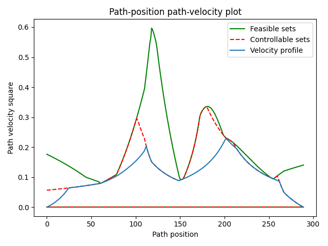
TOPP-RA: Time-Optimal Path Parameterization
Ruckig is a good fit when you need online motion from the current state to a target. TOPP-RA solves a related but different problem: you already have a geometric path, such as a spline through many waypoints, and you want to assign time optimally under velocity and acceleration constraints.
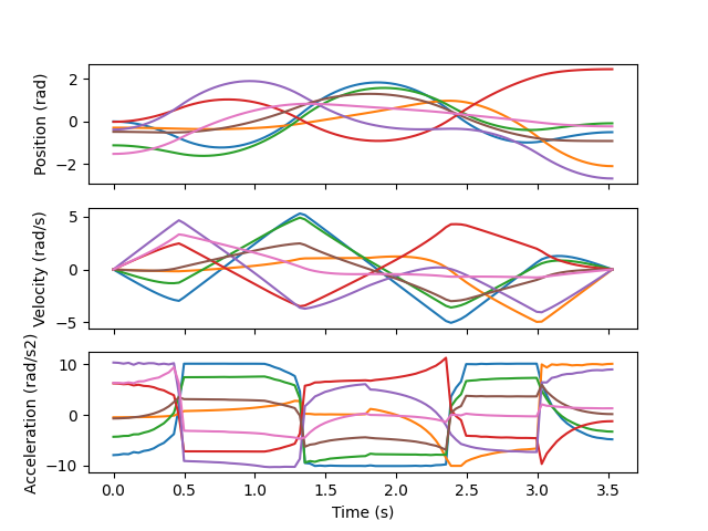
TOPP-RA uses reachable analysis to compute valid path velocity along the path parameter s. It is useful when a motion planner has already produced a collision-free path and you need to turn it into a trajectory:
Motion planner -> geometric path q(s)
TOPP-RA        -> time law s(t)
Controller     -> q(t), dq/dt, ddq/dt
The practical distinction:
| Problem | Good tool |
|---|---|
| Online servoing from current state to target with jerk limits | Ruckig |
| Offline or near-online time parameterization of a known path | TOPP-RA |
| Learning controller basics | Single-axis trapezoid or S-curve |
| Many waypoints, constraints and time optimization | TOPP-RA, then possibly jerk filtering |
The open-source TOPP-RA project traditionally focuses on velocity and acceleration constraints rather than online jerk-limited control. In a modern robot-arm controller, a pragmatic architecture is: let a planner create a geometric path, use TOPP-RA to parameterize or validate it, and use Ruckig or a servo layer for final jerk-limited updates.
Connecting Profiles to MoveJ, MoveL and Jogging
For MoveJ, time-scaling usually runs directly on joint deltas. The joint with the longest required motion often determines the duration, and the other joints are slowed down so all joints reach the target together. This is simple, stable and common in classical controllers.
For MoveL, the path is a Cartesian line. The profile should run on the line parameter s(t), then each control tick computes the TCP pose and calls IK to get joint commands. This preserves a straight TCP path, but you must still check joint velocity and acceleration after IK. If you only profile in Cartesian space and ignore joint limits, the robot can violate limits near singularities. The FK/IK/Jacobian and frames/jogging posts give the background.
For jogging, the target changes continuously as the operator moves a joystick or presses buttons. Trapezoids can feel abrupt when the operator starts and stops. S-curves or Ruckig are a better fit because each cycle can accept the current p/v/a, a new target or velocity intention, and jerk limits, then return a new state. This is why a jogging servo should usually be jerk-limited instead of using a hand-written velocity ramp.
Outside this series, ROS 2 remote monitoring is useful when you start logging profiles on real hardware, and AGV vs AMR shows why smooth profiles also matter outside fixed-base robot arms.
Selection Checklist
If you are building your first controller:
- Start with a trapezoid to validate FK/IK, interpolation and the command loop.
- Add an S-curve to understand jerk and reduce vibration.
- Use Ruckig for real online jerk-limited control.
- Use TOPP-RA or a similar path-parameterization tool when a planner already generated a geometric path.
- Always log
position/velocity/acceleration/jerkand compare them with motor and drive limits. - Test with the real payload at low speed before raising limits.
A common mistake is to only check the final position and declare the move correct. In motion control, the path to the final position is the critical part: peak velocity can exceed limits, acceleration can shake the gripper, jerk can excite resonance, and joints can finish at different times if synchronization is wrong.
Conclusion
The trapezoidal profile is the simplest useful starting point: easy to write, easy to debug, and good enough for many demonstrations. Its weakness is that acceleration changes discontinuously, so jerk is not bounded. The S-curve adds jerk limits, making motion smoother and closer to what a real robot arm needs.
If you are learning, write the Python prototype and C++ classes yourself. If you are building production control software, do not stop there: use Ruckig for online jerk-limited trajectory generation, and use TOPP-RA when you need to time-parameterize a geometric path from a planner. Used together, they provide a strong time-scaling layer for MoveJ, MoveL, blending, jogging and motion planning.