In the previous article on MoveJ and MoveL, we separated two core motion types: joint-space moves that get the robot to a target efficiently, and Cartesian linear moves that keep the TCP on a straight line. Real process work is not always straight. A glue bead around a rounded corner, a weld around a pipe opening, a polishing pass around a curved edge, or a camera orbit around a part all need circular or multi-point process motion.
Part 10 of this series focuses on two classic Cartesian commands:
- MoveC: move the TCP along a circular arc. The arc is defined by the current TCP pose, a via point, and a target point.
- MoveP: move along a process path through multiple waypoints, trying to keep TCP speed steady while using blend radii so the robot does not stop hard at each point.
The names are inspired by URScript, but the goal here is not vendor-specific programming. The goal is to build the controller logic yourself. By the end, you should understand how to fit a circle from three points, parameterize the arc, sample it by path length, solve IK for each sample, and sketch C++ functions such as moveC(via, to, v, a) and moveP(vector<pose>, v, blend) using Eigen.
1. What MoveC Actually Means
Let the three TCP positions be:
P0: the start point, which is the current TCP position.P1: the via point, an intermediate point that the arc must pass through.P2: the target point, where the circular segment ends.
If P0, P1, and P2 are not collinear, they define exactly one plane and exactly one circle on that plane. A MoveC command does not require the user to type the center of the circle. The controller infers the center, radius, plane normal, and arc direction from the three points. This is useful on a teach pendant because an operator can jog to a point on the curve and then to the end of the curve, instead of calculating center and angle by hand.
In URScript, the command shape is:
movec(pose_via, pose_to, a=1.2, v=0.25, r=0, mode=0)
Practical meaning:
pose_via: the second point on the circle; in fixed-orientation mode, the rotation part of this pose is usually not used.pose_to: the final point on the arc.a: TCP acceleration in m/s².v: TCP speed in m/s.r: blend radius at the target pose.mode=0: interpolate orientation from the current pose topose_to.mode=1: keep orientation fixed relative to the circular tangent.
The most important detail is that the first point on the circle is the current pose, not the first argument of movec. In normal programs, you first use MoveJ or MoveL to reach the arc start, then call MoveC.
2. Geometry Checks Before Fitting the Arc
MoveC looks simple from the operator side, but a controller has to reject bad inputs clearly. Three common issues appear again and again:
- The three points are almost collinear. The circle radius becomes huge, the plane normal becomes tiny, and the fit becomes noise-sensitive.
- The via point is too close to the start or target point. The resulting arc can be too small or require high directional acceleration.
- The TCP arc is geometrically valid but the robot cannot realize it because of singularities, joint limits, or collisions.
A practical controller should return errors such as ArcError::CollinearPoints, ArcError::RadiusTooSmall, or ArcError::IKFailedAtSample. For beginners, keep this mental model: MoveC is a geometry problem first, an IK problem second, and a timing problem third.
The basic geometry starts from two vectors:
u = P1 - P0
v = P2 - P0
n = u x v
If ||n|| is too small, the points are nearly collinear. Otherwise, n is the normal of the arc plane. The circle center is the intersection of two perpendicular bisectors on that plane: the bisector of segment P0-P1 and the bisector of segment P0-P2.
3. Python Prototype: Fit a Circle From Three Points
The Python prototype below intentionally avoids ROS and real robot drivers. It does three things: fits the circle, chooses the arc that passes through the via point, and plots the result. The IK function is a stub so you can replace it with the IK solver from the FK/IK/Jacobian article or your own library.
import numpy as np
import matplotlib.pyplot as plt

EPS = 1e-9

def normalize(x):
    n = np.linalg.norm(x)
    if n < EPS:
        raise ValueError("Vector is too small to normalize")
    return x / n

def circle_from_3_points(p0, p1, p2):
    p0 = np.asarray(p0, dtype=float)
    p1 = np.asarray(p1, dtype=float)
    p2 = np.asarray(p2, dtype=float)

    a = p1 - p0
    b = p2 - p0
    normal = np.cross(a, b)
    normal_norm = np.linalg.norm(normal)
    if normal_norm < 1e-6:
        raise ValueError("The three points are nearly collinear")
    normal = normal / normal_norm

    m01 = 0.5 * (p0 + p1)
    m02 = 0.5 * (p0 + p2)

    d01 = normalize(np.cross(normal, a))
    d02 = normalize(np.cross(normal, b))

    # Find s, t such that m01 + s*d01 is close to m02 + t*d02.
    A = np.column_stack([d01, -d02])
    rhs = m02 - m01
    s, t = np.linalg.lstsq(A, rhs, rcond=None)[0]
    center = m01 + s * d01
    radius = np.linalg.norm(p0 - center)
    return center, radius, normal

def angle_on_plane(point, center, e0, e1):
    r = point - center
    return np.arctan2(np.dot(r, e1), np.dot(r, e0))

def wrap_positive(theta):
    while theta < 0:
        theta += 2 * np.pi
    while theta >= 2 * np.pi:
        theta -= 2 * np.pi
    return theta

def arc_angles_through_via(p0, p1, p2, center, normal):
    e0 = normalize(p0 - center)
    e1 = normalize(np.cross(normal, e0))

    theta_via = wrap_positive(angle_on_plane(p1, center, e0, e1))
    theta_end = wrap_positive(angle_on_plane(p2, center, e0, e1))

    # Does the positive arc from 0 to theta_end contain the via point?
    if 0.0 <= theta_via <= theta_end:
        return 0.0, theta_end, e0, e1

    # Otherwise travel in the negative direction.
    if theta_end > 0:
        theta_end -= 2 * np.pi
    return 0.0, theta_end, e0, e1

def sample_movec(p0, p1, p2, ds=0.005):
    center, radius, normal = circle_from_3_points(p0, p1, p2)
    theta0, theta2, e0, e1 = arc_angles_through_via(p0, p1, p2, center, normal)

    arc_len = abs(theta2 - theta0) * radius
    n = max(2, int(np.ceil(arc_len / ds)) + 1)
    thetas = np.linspace(theta0, theta2, n)

    points = np.array([
        center + radius * (np.cos(t) * e0 + np.sin(t) * e1)
        for t in thetas
    ])
    return points, center, radius, normal

def ik_solve_stub(tcp_position, q_seed):
    # Replace with a real IK solver: analytic IK, DLS Jacobian, TRAC-IK,
    # Pinocchio, Robotics Toolbox, or your own implementation.
    return q_seed

p0 = np.array([0.45, -0.15, 0.32])
p1 = np.array([0.50,  0.00, 0.36])
p2 = np.array([0.42,  0.16, 0.32])

points, center, radius, normal = sample_movec(p0, p1, p2, ds=0.004)
q = np.zeros(6)
joint_path = []
for p in points:
    q = ik_solve_stub(p, q)
    joint_path.append(q)

fig = plt.figure(figsize=(9, 6))
ax = fig.add_subplot(111, projection="3d")
ax.plot(points[:, 0], points[:, 1], points[:, 2], label="MoveC arc")
ax.scatter(*p0, label="start P0", s=60)
ax.scatter(*p1, label="via P1", s=60)
ax.scatter(*p2, label="target P2", s=60)
ax.scatter(*center, label=f"center, r={radius:.3f} m", s=60)
ax.set_xlabel("x [m]")
ax.set_ylabel("y [m]")
ax.set_zlabel("z [m]")
ax.legend()
plt.tight_layout()
plt.show()
The arc-direction logic is the key part. There are two possible arcs between P0 and P2: one in the positive direction around the circle and one in the negative direction. The via point tells the controller which one to use. Many industrial systems also avoid representing a full circle with one MoveC command. If start and end are identical, one via point is not enough to uniquely define direction and number of turns, so full circles are often built from two circular moves.
4. TCP Speed and Sampling by Arc Length
If you sample by equal angle increments on a single circle, adjacent point spacing is nearly constant because ds = r * dtheta. For a basic MoveC generator, this is good enough. Timing can then follow the same idea from the trajectory types article: create a list of Cartesian waypoints, solve IK into joint waypoints, and assign timestamps using a velocity profile.
There is one important trap. Constant TCP speed does not automatically guarantee that every joint stays within velocity and acceleration limits. Near a singularity, a small TCP movement can require a large joint movement. A real controller should retime the joint trajectory or reduce the requested v if any segment violates qdot_max or qddot_max.
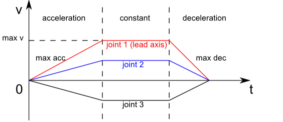
The plot above shows the basic velocity-profile idea. A Cartesian arc is similar: accelerate from zero to v, stay near constant speed in the middle, then decelerate to zero if the command does not blend into the next command. If there is a blend radius, the robot does not have to stop exactly at the target. It can leave the current segment early and connect smoothly to the next segment.
5. MoveP: Multi-Point Process Paths
MoveP is used for processes that care about steady TCP speed: gluing, dispensing, welding, polishing, coating, and similar tasks. Universal Robots describes MoveP as process motion that combines linear motion in tool space with circular blends, intended to keep tool speed constant. A smaller blend radius makes the corner sharper; a larger radius makes the path smoother but moves the TCP farther away from the nominal waypoint.
Imagine a path:
P0 -> P1 -> P2 -> P3 -> P4
If you execute this as MoveL commands with r=0, the robot slows down and stops at P1, P2, and P3. For glue dispensing, that creates blobs. MoveP blends around the corners. Before reaching P1, the robot leaves segment P0-P1, follows a small circular blend, and enters segment P1-P2. The TCP may not touch P1 exactly; it stays inside the blend region around P1.
For a beginner implementation, use this rule: blend must be smaller than half the length of the shortest adjacent segment. Otherwise, blend regions overlap. MoveIt Pro documents a similar requirement for Cartesian path following: the blending radius must be small enough to be applied at every waypoint.
6. C++ Eigen: Pose and MoveC Skeleton
The C++ code below is a minimal main.cpp. It does not drive hardware, but it generates sampled poses for MoveC and MoveP. Eigen is a good fit because Vector3d, cross(), dot(), and normalized() map directly to the 3D geometry.
#include <Eigen/Dense>
#include <cmath>
#include <iostream>
#include <stdexcept>
#include <vector>

using Vec3 = Eigen::Vector3d;

struct Pose {
  Vec3 p;
  Eigen::Quaterniond q;
};

struct Arc {
  Vec3 center;
  Vec3 normal;
  double radius;
};

static Vec3 normalizedChecked(const Vec3& v, const char* name) {
  const double n = v.norm();
  if (n < 1e-9) {
    throw std::runtime_error(std::string(name) + " is too small");
  }
  return v / n;
}

static Arc circleFrom3Points(const Vec3& p0, const Vec3& p1, const Vec3& p2) {
  const Vec3 a = p1 - p0;
  const Vec3 b = p2 - p0;
  Vec3 normal = a.cross(b);
  if (normal.norm() < 1e-6) {
    throw std::runtime_error("MoveC points are nearly collinear");
  }
  normal.normalize();

  const Vec3 m01 = 0.5 * (p0 + p1);
  const Vec3 m02 = 0.5 * (p0 + p2);
  const Vec3 d01 = normalizedChecked(normal.cross(a), "d01");
  const Vec3 d02 = normalizedChecked(normal.cross(b), "d02");

  Eigen::Matrix<double, 3, 2> A;
  A.col(0) = d01;
  A.col(1) = -d02;
  Eigen::Vector2d st = A.colPivHouseholderQr().solve(m02 - m01);

  Vec3 center = m01 + st(0) * d01;
  double radius = (p0 - center).norm();
  return {center, normal, radius};
}

static double wrapPositive(double x) {
  const double twoPi = 2.0 * M_PI;
  while (x < 0.0) x += twoPi;
  while (x >= twoPi) x -= twoPi;
  return x;
}

static double angleOnPlane(const Vec3& p, const Vec3& c, const Vec3& e0, const Vec3& e1) {
  Vec3 r = p - c;
  return std::atan2(r.dot(e1), r.dot(e0));
}

std::vector<Pose> moveC(const Pose& start, const Pose& via, const Pose& to,
                        double v, double a, double ds = 0.005) {
  (void)v;
  (void)a;
  Arc arc = circleFrom3Points(start.p, via.p, to.p);
  Vec3 e0 = normalizedChecked(start.p - arc.center, "arc e0");
  Vec3 e1 = normalizedChecked(arc.normal.cross(e0), "arc e1");

  double thetaVia = wrapPositive(angleOnPlane(via.p, arc.center, e0, e1));
  double thetaTo = wrapPositive(angleOnPlane(to.p, arc.center, e0, e1));
  if (!(0.0 <= thetaVia && thetaVia <= thetaTo)) {
    thetaTo -= 2.0 * M_PI;
  }

  double length = std::abs(thetaTo) * arc.radius;
  int n = std::max(2, static_cast<int>(std::ceil(length / ds)) + 1);

  std::vector<Pose> out;
  out.reserve(n);
  for (int i = 0; i < n; ++i) {
    double s = static_cast<double>(i) / static_cast<double>(n - 1);
    double theta = s * thetaTo;
    Pose pose;
    pose.p = arc.center + arc.radius * (std::cos(theta) * e0 + std::sin(theta) * e1);
    pose.q = start.q.slerp(s, to.q);
    out.push_back(pose);
  }
  return out;
}
The v and a arguments are not used for timestamping yet because this section focuses on geometry. In a real controller, the resulting std::vector<Pose> would go through IK, collision checks, joint-limit checks, and time parameterization. Keeping those layers separate makes debugging easier: if the TCP path is wrong, the bug is in geometry; if the TCP path is right but the robot jerks, the bug is probably in IK branch selection or retiming.
7. C++ Eigen: MoveP With Blend Radius
A full MoveP implementation can become complex, especially once you blend orientation, handle very short segments, and avoid collision. The beginner version below uses a clear approximation:
- Move in straight lines on each segment.
- At each middle waypoint, cut back by
blendon the incoming segment and forward byblendon the outgoing segment. - Connect the two cut points using a circular arc through the original waypoint.
static std::vector<Pose> sampleLine(const Pose& a, const Pose& b, double ds) {
  double length = (b.p - a.p).norm();
  int n = std::max(2, static_cast<int>(std::ceil(length / ds)) + 1);
  std::vector<Pose> out;
  for (int i = 0; i < n; ++i) {
    double s = static_cast<double>(i) / static_cast<double>(n - 1);
    Pose p;
    p.p = (1.0 - s) * a.p + s * b.p;
    p.q = a.q.slerp(s, b.q);
    out.push_back(p);
  }
  return out;
}

std::vector<Pose> moveP(const std::vector<Pose>& waypoints, double v,
                        double blend, double ds = 0.005) {
  if (waypoints.size() < 2) {
    throw std::runtime_error("MoveP needs at least two waypoints");
  }

  std::vector<Pose> path;
  Pose current = waypoints.front();

  for (size_t i = 1; i + 1 < waypoints.size(); ++i) {
    const Pose& prev = waypoints[i - 1];
    const Pose& corner = waypoints[i];
    const Pose& next = waypoints[i + 1];

    Vec3 dirIn = normalizedChecked(corner.p - prev.p, "MoveP dirIn");
    Vec3 dirOut = normalizedChecked(next.p - corner.p, "MoveP dirOut");
    double maxBlend = 0.45 * std::min((corner.p - prev.p).norm(), (next.p - corner.p).norm());
    double r = std::min(blend, maxBlend);

    Pose cutIn{corner.p - r * dirIn, corner.q};
    Pose cutOut{corner.p + r * dirOut, corner.q};

    auto line = sampleLine(current, cutIn, ds);
    path.insert(path.end(), line.begin(), line.end());

    auto arc = moveC(cutIn, corner, cutOut, v, /*a=*/1.0, ds);
    path.insert(path.end(), arc.begin(), arc.end());
    current = cutOut;
  }

  auto last = sampleLine(current, waypoints.back(), ds);
  path.insert(path.end(), last.begin(), last.end());
  return path;
}

int main() {
  Eigen::Quaterniond q = Eigen::Quaterniond::Identity();
  Pose p0{{0.35, -0.20, 0.30}, q};
  Pose p1{{0.45, -0.05, 0.34}, q};
  Pose p2{{0.42,  0.15, 0.34}, q};
  Pose p3{{0.30,  0.22, 0.31}, q};

  auto arc = moveC(p0, p1, p2, 0.10, 0.50);
  auto process = moveP({p0, p1, p2, p3}, 0.08, 0.03);

  std::cout << "MoveC samples: " << arc.size() << "\n";
  std::cout << "MoveP samples: " << process.size() << "\n";
  return 0;
}
Minimal CMakeLists.txt:
cmake_minimum_required(VERSION 3.16)
project(classical_arm_paths LANGUAGES CXX)

set(CMAKE_CXX_STANDARD 17)
set(CMAKE_CXX_STANDARD_REQUIRED ON)

find_package(Eigen3 3.4 REQUIRED NO_MODULE)

add_executable(paths main.cpp)
target_link_libraries(paths PRIVATE Eigen3::Eigen)
Build:
mkdir -p build
cmake -S . -B build
cmake --build build
./build/paths
8. From TCP Samples to Joint Commands
After you have TCP poses, the basic pipeline is:
- For each pose, solve IK using the previous solution as the seed.
- If IK fails, reduce
ds, switch IK branch, or reject the path. - Check joint limits and self-collision.
- Assign timestamps using a velocity profile.
- Send a
JointTrajectoryto the servo controller.
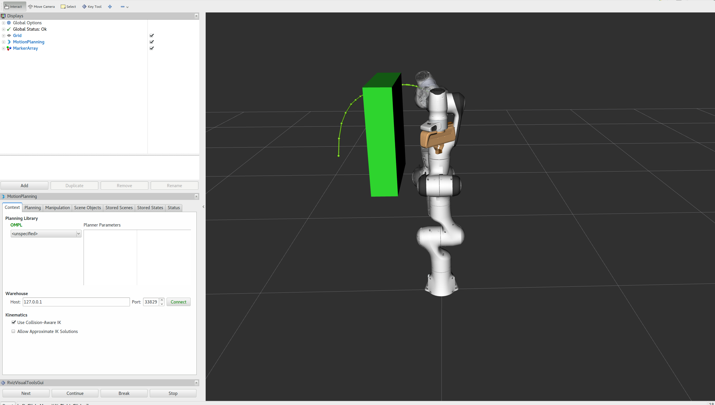
The MoveIt Cartesian path tutorial uses the same general idea: the user provides a list of end-effector waypoints, the system interpolates the Cartesian path with an eef_step, and then it creates a trajectory. For a small controller, you do not need to embed all of MoveIt, but its separation between waypoints, IK, path validation, and execution is worth copying.
9. Debug Checklist When the Arc Looks Wrong
If the circular path is not what you expected, check these items in order:
- Are
P0,P1, andP2expressed in the same frame? Mixing base frame and tool frame is common; review the frames and jogging article. - Are the three points nearly collinear?
- Is the via point on the side of the arc you intended?
- Are units meters or millimeters?
- Are you interpolating orientation to the target or keeping it relative to the tangent?
- Does IK jump between branches from one sample to the next?
- Is the blend radius too large for the distance between waypoints? See the blending article for the idea of blend regions and overlapping blends.
For process paths, the most common bug is choosing blend too large. The robot looks smooth, but it cuts the corner too aggressively, so the glue bead or weld seam drifts away from the part. Start with a small radius, plot the TCP path, measure maximum deviation, and only then increase the radius to reduce stops and vibration.
10. Exercises
- Modify the Python prototype to export
points.csv, one row perx,y,z. - Replace
ik_solve_stub()with the damped least-squares Jacobian IK from the previous article. - Plot
||q[i+1] - q[i]||to detect joint jumps. - Build a U-shaped MoveP path with five waypoints and test
blend = 0,0.01, and0.03. - Add a
max_tcp_deviationwarning when the blend cuts corners too much.
If you want to move toward production, the next step is integrating this path generator with collision checking and motion planning. You can read Open-RMF fleet management to see how larger systems separate planning, execution, and monitoring, or SLAM navigation robot to compare mobile robot path planning with Cartesian robot-arm path generation.
Sources
- Universal Robots, URScript
movec(pose_via, pose_to, a, v, r, mode)andmovep(pose, a, v, r): https://www.universal-robots.com/manuals/EN/PDF/SW10_7/scriptmanual_psx/script_directory_PolyscopeX.pdf - Universal Robots, Circular path using MoveP/MoveC: https://www.universal-robots.com/articles/ur/programming/circular-path-using-movepmovec/
- Universal Robots PolyScope Move node, MoveP process operation: https://www.universal-robots.com/manuals/EN/HTML/SW5_25/Content/prod-usr-man/software/PolyScope/content/BasicProgNodes/commandtab_move_en.htm
- MoveIt Tutorials, Cartesian path and RViz visualization: https://moveit.github.io/moveit_tutorials/
- MoveIt Pro Cartesian Path Following, blending radius constraint: https://docs.picknik.ai/6/how_to/cartesian_path_following/
- Eigen documentation, vector arithmetic and CMake imported target: https://libeigen.gitlab.io/eigen/docs-nightly/group__TutorialMatrixArithmetic.html