In the robot model article, we built forward kinematics: feed in joint vector q and get the TCP pose T_0e. In the inverse kinematics article, we used pose error to recover q. This article connects those two ideas through the most useful differential object in classical manipulation: the Jacobian.
If FK answers "where is the TCP for these joint angles?", the Jacobian answers a more immediate question: "if each joint moves with velocity qdot, what instantaneous velocity does the TCP get?". This is the foundation of Cartesian jogging, servoing, singularity avoidance, force control, and many industrial motion planners. By the end, you will derive the UR5 Jacobian by hand, implement J(q) in Python and C++, plot manipulability along a path, and convert Cartesian velocity commands into safe joint velocities.
1. What does the Jacobian map?
For a serial robot with n joints, the differential kinematic relation is:
twist_e = J(q) qdot
Here qdot is the n x 1 joint velocity vector. For a 6-DOF arm such as the UR5, J(q) is usually a 6 x 6 matrix. The first three rows are TCP linear velocity; the last three rows are angular velocity:
[vx vy vz wx wy wz]^T = J(q) [q1dot ... q6dot]^T
Modern Robotics describes the space/body Jacobian as the map from joint rates to an end-effector twist expressed in a chosen frame. Robotics Toolbox for Python states that robot.jacob0(q) is the geometric Jacobian in the world/base frame and maps joint velocity to end-effector spatial velocity. Pinocchio uses the same idea: getFrameJacobian returns a frame Jacobian, and the frame velocity is J * v.
The important distinction is:
| Type | Rotational output | Typical use |
|---|---|---|
| Geometric Jacobian | angular velocity omega = [wx, wy, wz] |
servoing, wrench/force mapping, resolved-rate control, singularity checks |
| Analytic Jacobian | derivative of orientation coordinates such as RPY, ZYZ Euler, exponential coordinates | pose interfaces that explicitly use a chosen orientation parameterization |
The translational part is the same, but the orientation part differs. The analytic Jacobian depends on the selected orientation representation, so it can become singular because of the representation itself, for example Euler-angle gimbal lock. For velocity controllers, prefer the geometric Jacobian for twist [v, omega], and convert to RPY/Euler rates only when the UI or planner requires it.
2. Hand-deriving revolute Jacobian columns for UR5
We will use the classic DH parameters for the UR5 CB-series:
| i | a_i (m) | d_i (m) | alpha_i |
|---|---|---|---|
| 1 | 0 | 0.089159 | pi/2 |
| 2 | -0.425 | 0 | 0 |
| 3 | -0.39225 | 0 | 0 |
| 4 | 0 | 0.10915 | pi/2 |
| 5 | 0 | 0.09465 | -pi/2 |
| 6 | 0 | 0.0823 | 0 |
Universal Robots publishes DH tables for UR models in its official support documentation. If you are using a UR5e, replace the a and d values with the UR5e row; the Jacobian formula below stays the same.
For each accumulated transform,
T_0i = A_1(q1) A_2(q2) ... A_i(qi)
extract:
p_i = T_0i[0:3, 3]
z_i = T_0i[0:3, 2]
For revolute joint i, the joint axis is z_{i-1} and the joint origin is p_{i-1}. If p_e is the TCP position, the Jacobian column is:
Jv_i = z_{i-1} x (p_e - p_{i-1})
Jw_i = z_{i-1}
J_i  = [Jv_i; Jw_i]
This is the most important formula in the article. It says that the linear velocity created by one rotating joint is the cross product between the joint axis and the vector from that joint to the TCP. The angular velocity contribution is the axis itself. If the joint were prismatic, the formula would become Jv_i = z_{i-1}, Jw_i = 0, but the UR5 has six revolute joints.
A quick intuition check: joint 1 rotates around the base z_0 axis. If the TCP is far from that axis, z_0 x (p_e - p_0) is large and the TCP moves quickly along a tangent. If the TCP is nearly above the base axis, joint 1 contributes little translational motion. That is the beginning of a shoulder singularity.
3. Singularity: when the Jacobian loses rank
A singularity occurs when J(q) is no longer full rank. For a 6 x 6 UR5 Jacobian, this means det(J) = 0, but in code a more stable test is the smallest singular value sigma_min approaching zero.
Common UR-style singularities:
| Type | Mechanical symptom | Control consequence |
|---|---|---|
| Wrist singularity | wrist is straight, often q5 near 0 or pi, and joint-4/joint-6 axes align |
one orientation direction is lost; q4 and q6 may need very high speeds |
| Shoulder singularity | wrist center is close to the joint-1 axis | the base cannot generate a desired lateral velocity direction |
| Elbow singularity | links 2 and 3 are nearly fully stretched or folded | the arm is near a workspace boundary and loses motion in one direction |
Do not rely only on det(J) in an online controller. It is sensitive to units and scaling. Use SVD instead:
J = U diag(sigma_1 ... sigma_m) V^T
sigma_min = min(sigma_i)
condition_number = sigma_max / sigma_min
manipulability = sqrt(det(J J^T))
The condition number is near 1 when the robot is isotropic: joint velocities can create TCP velocity reasonably evenly in all directions. When the condition number becomes large, the robot may still move, but one TCP direction is expensive: a small Cartesian velocity requires a large joint velocity. Yoshikawa's manipulability sqrt(det(JJ^T)) is proportional to the velocity ellipsoid volume; near zero, the ellipsoid collapses.
One practical warning: linear velocity is measured in m/s and angular velocity in rad/s. Full 6D manipulability is therefore scale-dependent. For TCP jogging along x/y/z, monitor the translational block Jv = J[0:3, :]. For full 6D pose control, scale angular rows by a characteristic length, such as 0.2 m, before comparing condition numbers.
4. Resolved-rate control
Resolved-rate motion control receives a Cartesian velocity command and solves for joint velocity:
qdot = J^+ v_des
If J is square and far from singularity, J^+ behaves like J^{-1}. If the robot is redundant or the task has fewer dimensions, J^+ is the Moore-Penrose pseudoinverse. For translational jogging, it is common to use Jv with shape 3 x 6:
qdot = Jv^+ [vx vy vz]^T
Near singularities, the pseudoinverse can explode because it divides by tiny singular values. Damped least squares (DLS) replaces it with:
J_dls^+ = J^T (J J^T + lambda^2 I)^-1
qdot    = J_dls^+ v_des
A larger lambda gives smoother, safer joint velocities, but worse TCP tracking. A useful rule is:
if sigma_min > sigma_safe: lambda = 0
else lambda = lambda_max * (1 - sigma_min / sigma_safe)^2
In a real controller, also clamp joint velocity, clamp acceleration, respect joint limits, and stop if sigma_min is too low while the operator keeps jogging into the dangerous direction.
5. Python from scratch: analytic J, numerical J, and TCP jogging
The script below is enough for a notebook: compare analytic Jacobian against numerical differentiation, plot manipulability along a simple path, and jog the TCP along x/y/z.
import numpy as np
import matplotlib.pyplot as plt

UR5_A = np.array([0.0, -0.425, -0.39225, 0.0, 0.0, 0.0])
UR5_D = np.array([0.089159, 0.0, 0.0, 0.10915, 0.09465, 0.0823])
UR5_ALPHA = np.array([np.pi / 2, 0.0, 0.0, np.pi / 2, -np.pi / 2, 0.0])

def dh(a, d, alpha, theta):
    c, s = np.cos(theta), np.sin(theta)
    ca, sa = np.cos(alpha), np.sin(alpha)
    return np.array([
        [c, -s * ca,  s * sa, a * c],
        [s,  c * ca, -c * sa, a * s],
        [0,      sa,      ca,     d],
        [0,       0,       0,     1],
    ], dtype=float)

def fk_all(q):
    T = np.eye(4)
    frames = [T.copy()]
    for a, d, alpha, theta in zip(UR5_A, UR5_D, UR5_ALPHA, q):
        T = T @ dh(a, d, alpha, theta)
        frames.append(T.copy())
    return frames

def fk(q):
    return fk_all(q)[-1]

def jacobian_analytic(q):
    frames = fk_all(q)
    pe = frames[-1][:3, 3]
    J = np.zeros((6, 6))
    for i in range(6):
        zi = frames[i][:3, 2]      # z_i, which is z_{i-1} in 1-based notation
        pi = frames[i][:3, 3]
        J[:3, i] = np.cross(zi, pe - pi)
        J[3:, i] = zi
    return J

def vee(S):
    return np.array([S[2, 1], S[0, 2], S[1, 0]])

def jacobian_numeric(q, eps=1e-6):
    T0 = fk(q)
    R0 = T0[:3, :3]
    J = np.zeros((6, 6))
    for i in range(6):
        dq = np.zeros(6)
        dq[i] = eps
        Tp = fk(q + dq)
        Tm = fk(q - dq)
        J[:3, i] = (Tp[:3, 3] - Tm[:3, 3]) / (2 * eps)

        Rdot = (Tp[:3, :3] - Tm[:3, :3]) / (2 * eps)
        omega_hat = Rdot @ R0.T          # spatial angular velocity
        J[3:, i] = vee(omega_hat)
    return J

def manipulability(J, rows=slice(0, 3)):
    A = J[rows, :]
    return np.sqrt(max(0.0, np.linalg.det(A @ A.T)))

def damped_pinv(J, lam):
    m = J.shape[0]
    return J.T @ np.linalg.inv(J @ J.T + (lam * lam) * np.eye(m))

def resolved_rate(q, twist, sigma_safe=0.05, lambda_max=0.2, qdot_limit=1.0):
    J = jacobian_analytic(q)
    s = np.linalg.svd(J, compute_uv=False)
    sigma_min = s[-1]
    lam = 0.0 if sigma_min >= sigma_safe else lambda_max * (1 - sigma_min / sigma_safe) ** 2
    qdot = damped_pinv(J, lam) @ twist
    qdot = np.clip(qdot, -qdot_limit, qdot_limit)
    return qdot, sigma_min, lam

q = np.deg2rad([0, -70, 90, -110, -90, 0])
Ja = jacobian_analytic(q)
Jn = jacobian_numeric(q)
print("max |Ja - Jn| =", np.max(np.abs(Ja - Jn)))

q0 = np.deg2rad([0, -90, 90, -90, -90, 0])
q1 = np.deg2rad([60, -60, 40, -110, -60, 30])
ts = np.linspace(0, 1, 200)
mu = []
kappa = []
for t in ts:
    q = (1 - t) * q0 + t * q1
    J = jacobian_analytic(q)
    s = np.linalg.svd(J, compute_uv=False)
    mu.append(manipulability(J, rows=slice(0, 3)))
    kappa.append(s[0] / max(s[-1], 1e-9))

plt.figure()
plt.plot(ts, mu, label="translational manipulability")
plt.twinx()
plt.plot(ts, kappa, "r", label="condition number")
plt.show()

q = q0.copy()
dt = 0.008
for _ in range(100):
    twist = np.array([0.03, 0.0, 0.0, 0.0, 0.0, 0.0])  # 3 cm/s along base X
    qdot, sigma_min, lam = resolved_rate(q, twist)
    q = q + qdot * dt
print("q final deg =", np.rad2deg(q))
If max |Ja - Jn| is large, the usual causes are DH multiplication order, using z_i instead of z_{i-1}, or computing the numerical angular velocity in the body frame while your analytic Jacobian is spatial. Debug column by column: perturb one joint and verify that the TCP moves in the expected tangent direction.
6. C++/Eigen: jacobian(q), SVD, and resolvedRate(twist)
Python is excellent for validation, but production servo loops often live in C++ or a ROS 2 node. This standalone Eigen skeleton mirrors the Python implementation:
// jacobian_demo.cpp
#include <Eigen/Dense>
#include <Eigen/SVD>
#include <algorithm>
#include <array>
#include <cmath>
#include <iostream>

using Vec6 = Eigen::Matrix<double, 6, 1>;
using Mat6 = Eigen::Matrix<double, 6, 6>;

const std::array<double, 6> A = {0.0, -0.425, -0.39225, 0.0, 0.0, 0.0};
const std::array<double, 6> D = {0.089159, 0.0, 0.0, 0.10915, 0.09465, 0.0823};
constexpr double PI = 3.14159265358979323846;
const std::array<double, 6> ALPHA = {PI / 2, 0.0, 0.0, PI / 2, -PI / 2, 0.0};

Eigen::Matrix4d dh(double a, double d, double alpha, double theta) {
  double c = std::cos(theta), s = std::sin(theta);
  double ca = std::cos(alpha), sa = std::sin(alpha);
  Eigen::Matrix4d T;
  T << c, -s * ca,  s * sa, a * c,
       s,  c * ca, -c * sa, a * s,
       0,      sa,      ca,     d,
       0,       0,       0,     1;
  return T;
}

std::array<Eigen::Matrix4d, 7> fkAll(const Vec6& q) {
  std::array<Eigen::Matrix4d, 7> frames;
  frames[0].setIdentity();
  for (int i = 0; i < 6; ++i) {
    frames[i + 1] = frames[i] * dh(A[i], D[i], ALPHA[i], q(i));
  }
  return frames;
}

Mat6 jacobian(const Vec6& q) {
  auto frames = fkAll(q);
  Eigen::Vector3d pe = frames[6].block<3, 1>(0, 3);
  Mat6 J;
  J.setZero();
  for (int i = 0; i < 6; ++i) {
    Eigen::Vector3d z = frames[i].block<3, 1>(0, 2);
    Eigen::Vector3d p = frames[i].block<3, 1>(0, 3);
    J.block<3, 1>(0, i) = z.cross(pe - p);
    J.block<3, 1>(3, i) = z;
  }
  return J;
}

Mat6 dampedPinv(const Mat6& J, double lambda) {
  Mat6 I = Mat6::Identity();
  return J.transpose() * (J * J.transpose() + lambda * lambda * I).inverse();
}

Vec6 resolvedRate(const Vec6& q, const Vec6& twist) {
  Mat6 J = jacobian(q);
  Eigen::JacobiSVD<Mat6> svd(J);
  auto s = svd.singularValues();
  double sigma_min = s(5);
  double sigma_safe = 0.05;
  double lambda_max = 0.2;
  double lambda = sigma_min >= sigma_safe ? 0.0
      : lambda_max * std::pow(1.0 - sigma_min / sigma_safe, 2.0);

  Vec6 qdot = dampedPinv(J, lambda) * twist;
  for (int i = 0; i < 6; ++i) {
    qdot(i) = std::clamp(qdot(i), -1.0, 1.0);
  }

  std::cout << "sigma_min=" << sigma_min << " lambda=" << lambda << "\n";
  return qdot;
}

int main() {
  Vec6 q;
  q << 0, -PI / 2, PI / 2, -PI / 2, -PI / 2, 0;
  Vec6 twist;
  twist << 0.03, 0, 0, 0, 0, 0;
  std::cout << resolvedRate(q, twist).transpose() << "\n";
}
cmake_minimum_required(VERSION 3.16)
project(ur5_jacobian_demo LANGUAGES CXX)

set(CMAKE_CXX_STANDARD 17)
set(CMAKE_CXX_STANDARD_REQUIRED ON)

find_package(Eigen3 REQUIRED)
add_executable(jacobian_demo jacobian_demo.cpp)
target_link_libraries(jacobian_demo Eigen3::Eigen)
Build:
mkdir -p build
cd build
cmake ..
cmake --build .
./jacobian_demo
For production, do not blindly call .inverse() in a high-rate loop without numerical checks. The version above is deliberately readable. In a real controller, build DLS from the SVD singular values, low-pass qdot, and stream sigma_min to telemetry.
7. Validate with libraries up to June 2026
Two libraries are especially useful for checking your from-scratch implementation:
Pinocchio 3.x
import pinocchio as pin

model = pin.buildModelFromUrdf("ur5.urdf")
data = model.createData()
q = pin.neutral(model)
frame_id = model.getFrameId("tool0")

pin.computeJointJacobians(model, data, q)
pin.updateFramePlacements(model, data)
J_pin = pin.getFrameJacobian(model, data, frame_id, pin.ReferenceFrame.LOCAL_WORLD_ALIGNED)
LOCAL_WORLD_ALIGNED is often convenient for controllers: the velocity is centered at the TCP frame origin, while the axes are aligned with the world/base frame. Pinocchio documentation notes that getFrameJacobian requires computeJointJacobians first; if q changes, recompute.
Robotics Toolbox for Python
import roboticstoolbox as rtb
import numpy as np

robot = rtb.models.UR5()
q = np.zeros(6)
J0 = robot.jacob0(q)              # geometric Jacobian in the base frame
Ja = robot.jacob0_analytical(q, "rpy/xyz")
When comparing against your DH code, make these identical: UR5 vs UR5e parameters, base/tool transforms, radians, reference frame, and row order [vx, vy, vz, wx, wy, wz]. Most Jacobian validation mismatches come from frame or tool-offset differences, not from the z x (p_e - p_i) formula itself.
8. Safety checklist for Cartesian jogging
Before connecting resolved-rate control to a real robot:
- Compare
J_analyticandJ_numericat at least 20 random poses. - Log
sigma_min, condition number, andmax(abs(qdot))every servo cycle. - Use DLS when
sigma_minis low; stop when it crosses a hard threshold. - Clamp
qdot, clampqdd, and respect joint-limit margins. - Scale orientation rows when mixing
m/sandrad/sin one norm. - Do not jog blindly through elbow, shoulder, or wrist singularities; slow down before dangerous regions.
- Test in simulation first, then run teach mode or very low speed on hardware.
If you read the frames and jogging article, pay special attention to the twist frame: jogging along base X is not the same as jogging along tool X. J is valid only when the twist and the Jacobian are expressed in the same frame.
When this controller becomes part of a larger system, you will need to connect it to a servo loop, command topics, and simulation. For the ROS 2 control architecture, see ROS 2 control for robots. For the test environment before touching real hardware, see the robotics simulation overview.
References
- Modern Robotics: Space Jacobian and Singularities
- Universal Robots: DH parameters
- Robotics Toolbox for Python:
jacob0()and analytic Jacobian - Pinocchio frame Jacobian docs
- Resolved-rate motion control overview