In the robot model article, we built forward kinematics: pass in a joint vector q and get the tool pose T_base_tool. In the FK/IK/Jacobian article, we saw that TCP velocity is related to joint velocity through v = J(q) qdot. This article turns those pieces into inverse kinematics: given a desired pose, find one or more joint configurations that reach it.
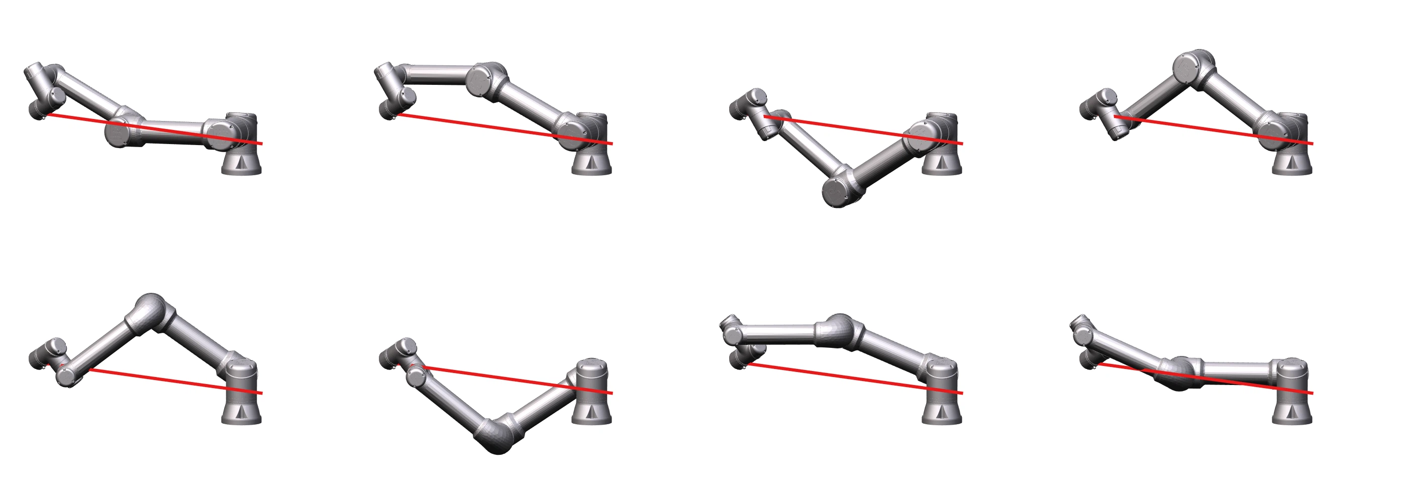
IK is where many robotics beginners get surprised. The same pose can have multiple solutions, no solution, or a solution that sits on a singularity. A 6-DOF UR5-like arm commonly has up to eight discrete solutions: shoulder left/right, elbow up/down, and wrist flip/non-flip. Once you add joint limits, self-collision, tool offset, cell constraints, and smooth motion requirements, the "right" answer is not just the one with the smallest residual. It is the one the controller can actually use.
What Should IK Return?
Forward kinematics is a function:
T = FK(q)
q = [q1, q2, q3, q4, q5, q6]^T
T ∈ SE(3)
Inverse kinematics asks for the reverse:
find q such that FK(q) ≈ T_target
The ≈ matters. Analytical IK tries to solve the trigonometry and algebra exactly. Numerical IK iterates until the residual is below a tolerance. In a real controller, the residual usually has six terms: three for position and three for orientation. A common form is:
e(q) = [ p_target - p(q) ]
       [ log(R(q)^T R_target) ]
log(R) is the small angle-axis vector for orientation error. If there is one beginner lesson to keep, keep this: do not subtract Euler angles directly unless you have carefully handled wrap-around and Euler singularities. For from-scratch code, start with a rotation vector or quaternion error.
A useful IK result object is explicit:
struct IKSolution {
    bool success;
    Eigen::VectorXd q;
    double residual_norm;
    int iterations;
    std::string reason;
};
An analytical solver should return a list, for example std::vector<Eigen::VectorXd>, because one target can have several valid branches. A numerical solver usually returns one solution near q0, so q0 is how you implicitly choose the branch.
Multiple Solutions, Joint Limits and Singularities
For an industrial 6R arm, multiple solutions come from geometric choices:
| Branch | Meaning |
|---|---|
| shoulder left/right | joint 1 reaches the target from two base-side configurations |
| elbow up/down | joints 2-3 form two different triangles to the wrist center |
| wrist flip | joint 5 changes sign while joints 4 and 6 compensate orientation |
Joint limits filter those solutions. A configuration can satisfy FK but exceed the mechanical range of q3, which makes it unusable. A configuration very close to a limit is also risky because the next MoveL or jogging command may run out of room. The numerical IK below therefore uses two layers: hard clamping after each step and a null-space term that gently pushes joints toward the center of their limits.
A singularity occurs when the Jacobian loses rank. At that point, a Cartesian velocity direction requires extremely large joint velocity, or one TCP direction cannot be controlled. UR-style arms often hit a wrist singularity when sin(q5) ≈ 0: wrist axes 4 and 6 align, so q4 and q6 are no longer uniquely separable. Analytical IK usually needs a q6_des from the previous configuration to keep the solution continuous. Numerical IK uses damped least squares so joint velocity does not explode.
By Hand: Closed-Form IK for UR5
We will use the familiar UR5 classic parameters from ur_kinematics:
d1 = 0.089159
a2 = -0.42500
a3 = -0.39225
d4 = 0.10915
d5 = 0.09465
d6 = 0.08230
Assume the desired pose is:
T = [ n_x  o_x  a_x  p_x ]
    [ n_y  o_y  a_y  p_y ]
    [ n_z  o_z  a_z  p_z ]
    [ 0    0    0    1   ]
The ROS ur_kinematics implementation flips a few matrix signs internally to match its convention. This section teaches the branch structure and equations; do not blindly paste signs into a project that uses a different DH table or URDF convention. Always validate with a round trip: q -> FK(q) -> IK(T) -> FK(q_ik).

Step 1: Solve theta1
Define:
A = d6 * T12 - T13
B = d6 * T02 - T03
R = A^2 + B^2
With the ur_kinematics convention, the two shoulder solutions are:
theta1_a = atan2(-B, A) + acos(d4 / sqrt(R))
theta1_b = atan2(-B, A) - acos(d4 / sqrt(R))
If d4^2 > R, the wrist center is inside an unreachable cylinder in the horizontal projection, so there is no real solution. Special cases such as A ≈ 0 or B ≈ 0 should be handled with clamped asin/acos to avoid numerical failure when a value becomes 1.0000000002.
Step 2: Solve theta5
For each theta1, solve wrist joint 2:
numer = T03 * sin(theta1) - T13 * cos(theta1) - d4
c5 = numer / d6
theta5_a = acos(clamp(c5, -1, 1))
theta5_b = 2*pi - theta5_a
This is the wrist-flip branch. If sin(theta5) is close to zero, the wrist is singular. The orientation around the tool axis is not uniquely determined; a practical controller should keep theta6 near its current value rather than letting the solution jump.
Step 3: Solve theta6
For each pair theta1, theta5, if abs(sin(theta5)) > eps:
theta6 = atan2(
    sign(sin(theta5)) * -(T01 * sin(theta1) - T11 * cos(theta1)),
    sign(sin(theta5)) *  (T00 * sin(theta1) - T10 * cos(theta1))
)
If sin(theta5) ≈ 0, use theta6_des from the current robot state. This is why an industrial analytical IK function often receives a seed or the current joint state even though the closed-form equations look independent.
Step 4: Solve theta2, theta3, theta4
Once theta1, theta5, and theta6 are known, the remaining part is a planar 3R problem. The ur_kinematics implementation computes:
x04x = -s5*(T02*c1 + T12*s1)
       -c5*(s6*(T01*c1 + T11*s1) - c6*(T00*c1 + T10*s1))

x04y = c5*(T20*c6 - T21*s6) - T22*s5

p13x = d5*(s6*(T00*c1 + T10*s1) + c6*(T01*c1 + T11*s1))
       -d6*(T02*c1 + T12*s1) + T03*c1 + T13*s1

p13y = T23 - d1 - d6*T22 + d5*(T21*c6 + T20*s6)
With p13x, p13y, joints 2-3 form a triangle with side lengths a2, a3:
c3 = (p13x^2 + p13y^2 - a2^2 - a3^2) / (2*a2*a3)
theta3_a = acos(clamp(c3, -1, 1))
theta3_b = 2*pi - theta3_a
If abs(c3) > 1, the target is outside the reach of the two main links. For each theta3, set:
denom = a2^2 + a3^2 + 2*a2*a3*cos(theta3)
A2 = a2 + a3*cos(theta3)
B2 = a3*sin(theta3)

theta2_a = atan2((A2*p13y - B2*p13x)/denom,
                 (A2*p13x + B2*p13y)/denom)

theta2_b = atan2((A2*p13y + B2*p13x)/denom,
                 (A2*p13x - B2*p13y)/denom)
Finally, theta4 accounts for the remaining orientation:
c23 = cos(theta2 + theta3)
s23 = sin(theta2 + theta3)

theta4 = atan2(c23*x04y - s23*x04x,
               x04x*c23 + x04y*s23)
The total is 2 shoulder choices × 2 wrist choices × 2 elbow choices = up to 8 solutions. Normalize them to [-pi, pi], filter joint limits, recompute FK for every candidate, and select the solution closest to q_current:
score(q) = w_pose * residual(q)
         + w_jump * ||wrap(q - q_current)||^2
         + w_limit * limit_penalty(q)

One Manual Newton/DLS Iteration
Numerical IK does not solve the global trigonometry. It linearizes FK around q_k:
e_k ≈ J(q_k) Δq
q_{k+1} = q_k + Δq
Newton/Gauss-Newton uses the pseudo-inverse:
Δq = J^+ e
J^+ = J^T (J J^T)^-1
Near a singularity, J J^T becomes close to singular. Damped least squares replaces it with:
Δq = J^T (J J^T + λ^2 I)^-1 e
A single hand calculation looks like this:
e = [0.010, -0.004, 0.006, 0.020, 0.000, -0.010]^T
||e|| = 0.025 m/rad-mixed
λ = 0.03
solve (J J^T + λ^2 I) y = e
Δq = J^T y
q_next = clamp(q + α Δq, q_min, q_max)
α is the step scale, often between 0.2 and 1.0. If the residual grows, reduce α or increase λ. In a well-conditioned region, a small λ gives fast convergence; near a singularity, a larger λ makes the step conservative.
From Scratch: Python Prototype
The Python prototype should be short, easy to plot, and use the same FK/Jacobian convention as the C++ project. The code below assumes fk(q) returns R, p and jacobian(q) returns a 6×6 geometric Jacobian in the base frame.
import numpy as np
import matplotlib.pyplot as plt

def so3_error(R, Rd):
    Rerr = R.T @ Rd
    return 0.5 * np.array([
        Rerr[2, 1] - Rerr[1, 2],
        Rerr[0, 2] - Rerr[2, 0],
        Rerr[1, 0] - Rerr[0, 1],
    ])

def ik_dls(target_R, target_p, q0, q_min, q_max,
           lam=0.03, alpha=0.6, tol=1e-5, max_iter=200):
    q = q0.copy()
    mid = 0.5 * (q_min + q_max)
    span = q_max - q_min
    hist = []

    for it in range(max_iter):
        R, p = fk(q)
        e = np.r_[target_p - p, so3_error(R, target_R)]
        hist.append(np.linalg.norm(e))
        if hist[-1] < tol:
            return q, True, np.array(hist)

        J = jacobian(q)
        A = J @ J.T + (lam * lam) * np.eye(6)
        dq_task = J.T @ np.linalg.solve(A, e)

        # Null-space: push joints gently toward the center of their limits.
        J_pinv = J.T @ np.linalg.solve(A, np.eye(6))
        N = np.eye(len(q)) - J_pinv @ J
        grad_limit = -2.0 * (q - mid) / (span * span)
        dq = dq_task + 0.05 * (N @ grad_limit)

        q = np.clip(q + alpha * dq, q_min, q_max)

    return q, False, np.array(hist)

q_sol, ok, residual = ik_dls(Rd, pd, q0, q_min, q_max)
plt.semilogy(residual)
plt.xlabel("iteration")
plt.ylabel("||residual||")
plt.grid(True)
plt.show()
The so3_error skew approximation above is fine for small orientation errors. If the target is far away, use the full SO(3) logarithm map. This article keeps the prototype beginner-friendly so the IK loop is easy to see.
From Scratch: C++/Eigen numericalIK
In the runtime path, we do not plot. We return a clear status:
struct IKOptions {
    int max_iter = 100;
    double tolerance = 1e-5;
    double lambda = 0.03;
    double alpha = 0.7;
    double null_gain = 0.05;
};

struct IKResult {
    bool success = false;
    Eigen::VectorXd q;
    double residual_norm = 0.0;
    int iterations = 0;
};
Here is a compact DLS implementation:
IKResult numericalIK(const Eigen::Isometry3d& target,
                     const Eigen::VectorXd& q0,
                     const Eigen::VectorXd& q_min,
                     const Eigen::VectorXd& q_max,
                     const IKOptions& opt) {
    Eigen::VectorXd q = q0;
    const int n = q.size();
    const Eigen::VectorXd mid = 0.5 * (q_min + q_max);
    const Eigen::VectorXd span = q_max - q_min;

    IKResult out;
    out.q = q;

    for (int iter = 0; iter < opt.max_iter; ++iter) {
        Eigen::Isometry3d T = forwardKinematics(q);
        Eigen::Matrix<double, 6, 1> e;
        e.head<3>() = target.translation() - T.translation();
        Eigen::AngleAxisd aa(T.rotation().transpose() * target.rotation());
        e.tail<3>() = T.rotation() * (aa.axis() * aa.angle());

        const double norm = e.norm();
        if (norm < opt.tolerance) {
            out.success = true;
            out.q = q;
            out.residual_norm = norm;
            out.iterations = iter;
            return out;
        }

        Eigen::MatrixXd J = geometricJacobian(q);  // 6 x n
        Eigen::Matrix<double, 6, 6> A =
            J * J.transpose()
            + opt.lambda * opt.lambda * Eigen::Matrix<double, 6, 6>::Identity();

        Eigen::MatrixXd Jpinv = J.transpose() * A.ldlt().solve(
            Eigen::Matrix<double, 6, 6>::Identity());
        Eigen::VectorXd dq_task = Jpinv * e;

        Eigen::MatrixXd N = Eigen::MatrixXd::Identity(n, n) - Jpinv * J;
        Eigen::VectorXd grad_limit =
            -2.0 * (q - mid).array() / span.array().square();
        Eigen::VectorXd dq = dq_task + opt.null_gain * (N * grad_limit);

        q += opt.alpha * dq;
        q = q.cwiseMax(q_min).cwiseMin(q_max);
        out.residual_norm = norm;
        out.iterations = iter + 1;
    }

    out.q = q;
    return out;
}
For n = 6, the null-space term has limited effect because the task consumes all six degrees of freedom, although damping still leaves a soft projection. For a 7-DOF arm or a mobile manipulator, the same structure becomes much more useful. Keeping it from the start makes the project easier to extend.
Minimal CMakeLists.txt:
cmake_minimum_required(VERSION 3.16)
project(arm_controller_ik LANGUAGES CXX)

set(CMAKE_CXX_STANDARD 17)
set(CMAKE_CXX_STANDARD_REQUIRED ON)

find_package(Eigen3 REQUIRED)

add_library(arm_controller
    src/robot_model.cpp
    src/kinematics.cpp
    src/numerical_ik.cpp
)

target_include_directories(arm_controller PUBLIC include)
target_link_libraries(arm_controller PUBLIC Eigen3::Eigen)

add_executable(test_ik tests/test_ik_roundtrip.cpp)
target_link_libraries(test_ik PRIVATE arm_controller)
Round-trip test:
int main() {
    Eigen::VectorXd q(6);
    q << 0.2, -1.1, 1.4, -0.6, 0.8, 0.3;

    Eigen::VectorXd q_min(6), q_max(6);
    q_min.setConstant(-M_PI);
    q_max.setConstant(M_PI);

    Eigen::Isometry3d target = forwardKinematics(q);
    IKOptions opt;
    IKResult sol = numericalIK(target, q + Eigen::VectorXd::Constant(6, 0.05),
                               q_min, q_max, opt);

    Eigen::Isometry3d check = forwardKinematics(sol.q);
    double pos_err = (target.translation() - check.translation()).norm();
    Eigen::AngleAxisd aa(check.rotation().transpose() * target.rotation());

    if (!sol.success || pos_err > 1e-4 || std::abs(aa.angle()) > 1e-4) {
        return 1;
    }
    return 0;
}
Build:
cmake -S . -B build -G Ninja
cmake --build build
./build/test_ik
Libraries Worth Knowing, Updated to 2026-06-13
Robotics Toolbox for Python remains one of the easiest libraries for learning and checking manipulator kinematics. robot.ikine_LM(...) is a Levenberg-Marquardt numerical IK method with q0, tol, joint_limits, mask, ilimit, slimit, and limit/manipulability options. PyPI currently lists roboticstoolbox-python as version 1.1.1, uploaded on 2024-05-11.
Pinocchio is a strong C++/Python library for rigid-body algorithms. The Pinocchio CLIK example shows the classic loop: load the model, run forward kinematics, compute frame error, compute the Jacobian, solve a damped velocity step, then call integrate(model, q, v*dt). If your project is pinned to Pinocchio 3.x, the CLIK pattern is still a good reference. The latest state checked on 2026-06-13 is different: PyPI package pin is 4.0.0, uploaded on 2026-05-21, and the latest GitHub release is also v4.0.0.
Pink is differential IK on top of Pinocchio. PyPI pin-pink is currently 4.2.0, released on 2026-04-20. Its strength is the weighted task/limit model: frame tasks, posture tasks, center-of-mass tasks, joint limits, and barriers. If you move from a single arm to a humanoid or mobile manipulator, the "many tasks + QP" formulation scales better than a one-target DLS loop.
Mink is differential IK on top of MuJoCo. PyPI mink is currently 1.1.1, released on 2026-05-15. It computes joint velocity from task-space objectives and constraints through a QP, which makes it useful for MuJoCo simulation, teleoperation, and motion retargeting.
NVIDIA cuRobo is a CUDA library for motion generation, including forward/inverse kinematics, collision checking, trajectory optimization, geometric planning, and whole-body motion generation. The latest GitHub release checked on 2026-06-13 is v0.8.0, named "cuRoboV2 research and Open Source", published on 2026-04-18. It is not the beginner replacement for the small C++ solver in this article, but it is important when you need to run many IK/planning seeds in parallel on a GPU.
IK Debug Checklist
If IK does not converge, check in this order:
- Is FK correct? Use a known
qand compare against Robotics Toolbox or Pinocchio. - Is the Jacobian expressed in the same frame as the residual? A base-frame residual with a tool-frame Jacobian will behave badly.
- Is the orientation error direction correct? Try solving position only first.
- Are units consistent: radians and metres?
- Is the target inside the workspace and inside joint limits?
- Are you near a singularity? Print
det(JJ^T)or the singular values ofJ. - Is the seed
q0near the branch you want?
Analytical IK is fast and can return every branch, which is ideal for UR-style arms and discrete pose targets. Numerical IK is more flexible: it works with arbitrary URDFs, tool offsets, redundant robots, and secondary tasks. A practical classical controller often uses both: analytical IK to enumerate good candidates when the robot has a known formula, numerical IK/DLS to refine and handle continuous MoveL or jogging targets, and library solvers when the robot model grows beyond a clean 6R arm.
References
- Kelsey P. Hawkins, "Analytic Inverse Kinematics for the Universal Robots UR-5/UR-10 Arms", Georgia Tech, 2013.
- ROS Industrial
ur_kinematics,ur_kin.cpp, for UR5 parameters and branch IK. - Alexander Elias, "UR5 Inverse Kinematics" and
aelias36/ik-geo-ur5. - Robotics Toolbox for Python documentation:
Robot.ikine_LM. - Pinocchio documentation: inverse kinematics CLIK example.
- Pink 4.2.0 documentation and PyPI
pin-pink. - Mink documentation and PyPI
mink. - NVIDIA cuRobo GitHub and Isaac Sim cuRobo documentation.