Introduction: From Idea to Implementation
In Part 1, we understood why SimpleVLA-RL matters: it breaks through the SFT performance ceiling by letting VLA models practice with binary rewards. Now it's time to answer how — what architecture, what algorithm, and what engineering decisions make this system work.
This post dives deep into three technical pillars: (1) the OpenVLA-OFT backbone and its token-based action representation, (2) the GRPO algorithm with asymmetric clipping, and (3) dynamic sampling — a technique that seems simple but determines the success or failure of the entire system.
Backbone: OpenVLA-OFT
Architecture Overview
SimpleVLA-RL is built on OpenVLA-OFT (Open Vision-Language-Action with Optimal Fine-Tuning), an improved variant of the original OpenVLA. The architecture consists of:
- Language Model: LLaMA2-7B as the central "brain," processing both language and actions
- Vision Encoders: Two parallel encoders:
- SigLIP for semantic features (understanding "this is a cup")
- DINOv2 for spatial features (understanding "the cup is at coordinates (x, y, z)")
- Action Head: Converts LLaMA's output into 7-DoF robot actions
The workflow: camera images pass through both vision encoders, features are concatenated and projected into LLaMA2's embedding space. Combined with a natural language task instruction (e.g., "pick up the red cup"), LLaMA2 generates a sequence of action tokens.
Token-based Actions: Why Not Regression?
This is the critical design decision, and it determines the feasibility of applying RL.
Traditional approach (regression): The action head directly outputs 7 continuous values (6-DoF pose + gripper). Uses loss functions like L1 or MSE. The original OpenVLA-OFT uses an MLP head with L1 loss.
SimpleVLA-RL's approach (token-based): Each action dimension is discretized into bins, then represented as tokens — exactly like how LLMs generate text. Each action step produces 256 tokens. Action chunking groups multiple steps into one sequence:
- LIBERO: chunk size = 8 steps, yielding 8 x 256 = 2048 tokens
- RoboTwin: chunk size = 25 steps, yielding 25 x 256 = 6400 tokens
Why is token-based critical for RL? Three reasons:
-
Natural probability distributions: Each token has a probability distribution over the vocabulary, enabling log-probability computation — the core component of policy gradients. With regression output, you must assume a distribution (Gaussian), and that assumption is often incorrect.
-
GRPO compatibility: GRPO (and PPO, REINFORCE, etc.) needs to compute the ratio pi(a|s)/pi_old(a|s). With token-based actions, this ratio computes naturally through autoregressive generation. With regression, you need to parameterize a separate distribution.
-
Natural exploration: Increasing the temperature when sampling tokens automatically increases exploration — no need for separate noise injection. At temperature 1.6, the model is "creative" enough to try novel actions.
Comparison with Original OpenVLA-OFT
| Feature | Original OpenVLA-OFT | SimpleVLA-RL Version |
|---|---|---|
| Action representation | MLP head, continuous | Token-based, discrete |
| Loss function | L1 regression | Cross-entropy (SFT), GRPO (RL) |
| Camera views | Multi-view | Single-view (reduced complexity) |
| RL compatible? | Difficult (needs distribution head) | Yes, naturally |
The switch to single-view is also noteworthy. Multi-view provides better 3D information, but single-view dramatically reduces computational cost for RL rollouts — and with sufficient training data, single-view achieves comparable performance.
GRPO: The Optimization Algorithm
What is Group Relative Policy Optimization?
GRPO (Group Relative Policy Optimization) was originally developed for RLHF in LLMs (by the DeepSeek team), and SimpleVLA-RL is one of the first works to apply it to robot manipulation.
The core idea: instead of using a separate critic network to estimate the value function (like PPO), GRPO computes advantages relative to the group — comparing trajectories against each other.
How GRPO Works, Step by Step
Step 1: Sampling. For each query (initial state + task instruction), the model generates G = 8 different trajectories (enabled by high temperature). Each trajectory is a sequence of action tokens.
Step 2: Evaluate. Execute all 8 trajectories in simulation, assigning binary rewards:
# Pseudocode
rewards = []
for trajectory in trajectories:
    success = env.evaluate(trajectory)
    rewards.append(1.0 if success else 0.0)
# Example: rewards = [1, 0, 1, 1, 0, 0, 1, 0]
Step 3: Compute group-relative advantage. Normalize rewards within the group:
mean_r = mean(rewards)   # = 0.5
std_r = std(rewards)     # approx 0.535
advantages = [(r - mean_r) / std_r for r in rewards]
# Successful trajectories get positive advantage, failures get negative
Step 4: Policy update. Maximize the objective:
L = E[ min(ratio * A, clip(ratio, 1-eps_low, 1+eps_high) * A) ]
Where:
ratio = pi_new(a|s) / pi_old(a|s)— probability ratio between new and old policyA— advantage from step 3eps_low = 0.2,eps_high = 0.28— asymmetric clipping bounds
Asymmetric Clipping: A Subtle but Powerful Technique
This is one of the most important technical contributions. In standard PPO, clipping is symmetric: [1-eps, 1+eps] with eps = 0.2, giving [0.8, 1.2]. SimpleVLA-RL uses asymmetric clipping: [0.8, 1.28].
Why? Consider a concrete scenario:
-
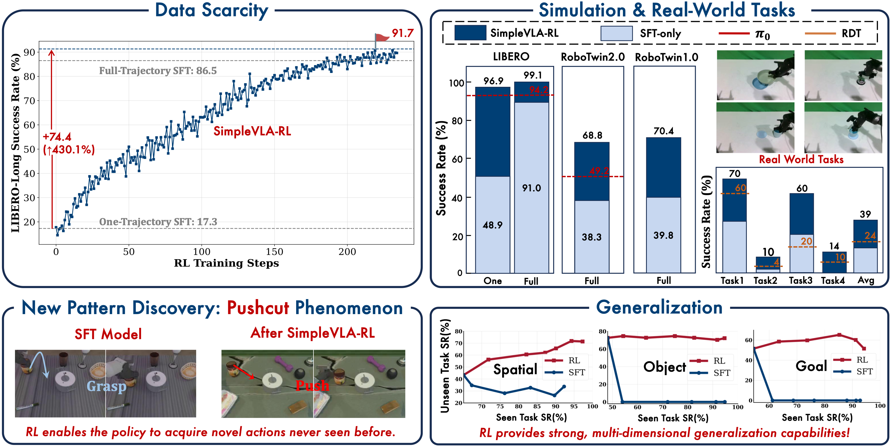
Rare but successful actions: An action that the old policy assigned very low probability (e.g., pushing instead of grasping) but led to success. The ratio is large (pi_new >> pi_old). With symmetric clipping, the ratio is capped at 1.2 — the policy only "gently" increases the probability. With asymmetric clipping (capped at 1.28), the policy can increase the probability more aggressively for good actions it hadn't tried before.
-
Common but failed actions: The ratio is small (pi_new < pi_old). Clipping at 0.8 — decrease probability, but not too fast to avoid losing diversity.
In simple terms: eps_high > eps_low means "increase faster than decrease" — encouraging stronger exploration, which is especially important when binary reward creates weak gradient signals.
No KL Divergence: Radical Simplification
Traditional PPO often adds a KL penalty to prevent the new policy from diverging too far from the old one:
L = L_clip - beta * KL(pi_new || pi_old)
SimpleVLA-RL completely removes the KL term (beta = 0). The reasoning:
- GPU memory savings: No need to store the reference model (7B parameters), saving approximately 14GB VRAM per GPU.
- SFT provides a good base: After SFT, the VLA model already has a "reasonable" policy — it knows how to approach objects and move the gripper. RL only needs fine-tuning, not drastic changes. The clipping bound is sufficient to prevent policy divergence.
- Empirical evidence: Experiments show that adding KL doesn't improve results and can actually decrease performance by limiting exploration.

Dynamic Sampling: Simple Yet Decisive
The Problem: Vanishing Gradients
Recall Step 3 — computing advantages. If all 8 trajectories succeed (rewards = [1,1,1,1,1,1,1,1]), then:
mean_r = 1.0
std_r = 0.0  # All identical!
advantages = [0, 0, 0, 0, 0, 0, 0, 0]  # No signal!
The same happens if all trajectories fail. When advantage = 0 for every trajectory, gradient = 0, and the model learns nothing.
This is especially severe with binary reward. With dense reward (0.1, 0.3, 0.7, 0.9), even if all trajectories succeed, advantages are still non-zero because rewards differ. But binary reward has only 2 values, so the probability of a uniform batch is very high.
The Solution: Discard Uniform Batches
SimpleVLA-RL applies dynamic sampling: for each batch, if all trajectories have the same reward (all-success or all-fail), discard the batch and resample.
# Pseudocode
while True:
    trajectories = model.generate(query, num_samples=8, temperature=1.6)
    rewards = [env.evaluate(t) for t in trajectories]

    if len(set(rewards)) > 1:  # Mix of successes and failures
        break  # This batch is useful
    # Otherwise, resample
This technique sounds simple, but without it, RL training completely fails. The paper's ablation shows that removing dynamic sampling drops performance by 15-20% compared to having it.
The Intuition
Think of dynamic sampling as selecting exercises at the right difficulty level. If you always solve problems that are too easy (all-success), you don't learn anything new. If you always face problems that are too hard (all-fail), you don't learn either. You learn the most when problems are at the boundary between possible and impossible — and that's exactly what dynamic sampling ensures.
Temperature: Balancing Exploration and Exploitation
SimpleVLA-RL uses temperature = 1.6 when generating trajectories (rollout), and temperature = 0 (greedy) during inference.
Why 1.6?
Temperature 1.0 is the "default" — the probability distribution stays as-is from the model. Temperature > 1.0 flattens the distribution, increasing the probability of less common tokens. At temperature 1.6:
- The most common token (e.g., "move downward") still has the highest probability
- But less common tokens (e.g., "push left") have significantly higher probability compared to temperature 1.0
- Result: the model tries many different strategies instead of repeating the same approach
Temperature 1.6 is the sweet spot — high enough to explore, but not so high that actions become completely random (temperature > 2.0 is usually too noisy).
Two Operating Modes
| Phase | Temperature | Purpose |
|---|---|---|
| Training (rollout) | 1.6 | Maximum exploration, collecting diverse trajectories |
| Inference (deploy) | 0 (greedy) | Maximum exploitation, selecting the best action |
This separation matters: training and inference have different objectives. Training needs diversity to discover new strategies. Inference needs consistency to achieve the highest success rate.
Binary Reward: Simple but Sufficient
Reward Applied to the Entire Trajectory
An important detail: the reward R = 1 or R = 0 is assigned to all tokens in the trajectory, not just the last token. This means:
# If trajectory succeeds
token_rewards = [1, 1, 1, 1, ..., 1]  # All tokens receive R=1

# If trajectory fails
token_rewards = [0, 0, 0, 0, ..., 0]  # All tokens receive R=0
Why not assign reward to individual tokens? Because we don't know which token matters. In a trajectory of 2048 tokens, token #500 (the decision to push instead of grasp) might be the determining factor, but we have no way of knowing. By assigning the same reward to all tokens, GRPO will automatically figure out which tokens' probabilities to increase or decrease through group-relative advantages.
Comparison with Dense Reward
| Feature | Binary Reward | Dense Reward |
|---|---|---|
| Design effort | Automatic (task success detector) | Requires expert design per task |
| Reward hacking | Very difficult to exploit | Easily exploitable |
| Gradient signal | Weak (needs dynamic sampling) | Strong |
| Generalization | High (task-agnostic) | Low (task-specific) |
| Scalability | Excellent | Poor (must redesign per task) |
Binary reward trades off weaker gradient signal for scalability and robustness — and combined with dynamic sampling, this drawback is effectively mitigated.
Data Flow: End to End
Let's trace a complete training loop:
1. Query Generation: Select a task (e.g., "pick up the red cup") and a random initial state in simulation.
2. Rollout: VLA model generates 8 trajectories in parallel, each consisting of:
- Input: camera image + task instruction
- Output: action token sequence (2048 for LIBERO)
- Temperature: 1.6
3. Execution: Each trajectory is executed in the simulation environment (LIBERO/RoboTwin).
4. Reward Assignment: Check task completion, assign R = 1 or 0.
5. Dynamic Sampling Check: If all rewards are identical, discard the batch and return to step 1. If there's a mix of 0s and 1s, continue.
6. Advantage Computation: Normalize rewards within the group to get advantages.
7. Policy Update: GRPO update with asymmetric clipping.
8. Repeat: Return to step 1 with the updated policy.
The entire process runs on 8 NVIDIA A800 80GB GPUs, using the veRL framework (v0.2) to parallelize rollout and training.
GRPO vs PPO Comparison
| Feature | PPO | GRPO |
|---|---|---|
| Critic network | Required (extra parameters, training) | Not needed |
| KL regularization | Commonly used | Not needed |
| Advantage estimation | GAE (needs value function) | Group-relative (compare within batch) |
| Memory footprint | High (policy + critic + ref model) | Low (policy only) |
| Hyperparameters | Many (GAE lambda, critic LR, KL beta, ...) | Few (eps_low, eps_high, temperature) |
| Implementation complexity | High | Medium |
GRPO trades accuracy of advantage estimation (PPO's learned critic is more precise) for simplicity and efficiency. With a 7B parameter VLA model, removing the critic network saves approximately 14GB VRAM — enough to increase batch size or reduce the number of GPUs needed.
Key Hyperparameters
Here's a summary of SimpleVLA-RL's key hyperparameters:
| Parameter | Value | Meaning |
|---|---|---|
| Learning rate | 5e-6 | Low to prevent catastrophic forgetting |
| Batch size | 64 | Queries per iteration |
| Samples per query | 8 | Parallel trajectories |
| eps_low (clip) | 0.2 | Lower bound for probability decrease |
| eps_high (clip) | 0.28 | Upper bound for probability increase |
| Temperature (rollout) | 1.6 | Exploration level |
| Temperature (inference) | 0.0 | Greedy, no exploration |
| KL coefficient | 0.0 | KL not used |
| Action tokens per step | 256 | Discretized 7-DoF action |
| Chunk size (LIBERO) | 8 | Action steps per prediction |
| Chunk size (RoboTwin) | 25 | More steps for dual-arm |
| GPUs | 8x A800 80GB | Training hardware |
The learning rate of 5e-6 is noteworthy — much lower than typical SFT (1e-4). The reason: RL training can easily cause catastrophic forgetting — the model forgets SFT knowledge if updates are too aggressive. A low learning rate ensures the model improves gradually without destroying its foundation.

Setup: How to Reproduce
If you want to reproduce SimpleVLA-RL results, here's the basic setup:
# Environment
conda create -n simplevla python=3.10
conda activate simplevla

# Core dependencies
pip install torch==2.4.0 --index-url https://download.pytorch.org/whl/cu124
pip install flash-attn==2.5.8
pip install verl==0.2

# Clone repos
git clone https://github.com/PRIME-RL/SimpleVLA-RL
git clone https://github.com/moojink/openvla-oft

# Install
cd SimpleVLA-RL && pip install -e .
Minimum hardware requirements: 8x A800/H100 80GB GPUs. This is the biggest barrier — not every lab has access to an 8-GPU high-end cluster. However, the community is working on LoRA + gradient checkpointing versions to run on 2-4 GPUs.
To learn more about setting up LeRobot for similar experiments, check out our AI for Robotics series.
Architectural Lessons
Looking at SimpleVLA-RL's design holistically, several important lessons emerge:
1. Token-based > Regression for RL
Switching from regression to token-based actions isn't just a technical detail — it unlocks the ability to apply RL. This is a textbook example of representation determines algorithm: choosing the right data representation matters more than choosing the right algorithm.
2. Simple > Complex
No KL, no critic, no dense reward — each omission has a clear rationale, and ablation studies confirm that removing them doesn't hurt performance. The lesson: always start with the simplest solution, only adding complexity when there's evidence it's needed.
3. RL Tailored for VLA
Unlike RL for games (dense rewards, short episodes), RL for robot manipulation has unique characteristics: sparse rewards, long trajectories, continuous state spaces. SimpleVLA-RL shows that rather than forcing traditional RL frameworks onto robotics, adapting the framework to fit (binary reward + dynamic sampling + asymmetric clipping) produces better results.
Limitations and Future Directions
Despite its impressive results, SimpleVLA-RL has limitations worth acknowledging:
-
Large hardware requirements: 8x A800 GPUs aren't available in every lab. More research is needed on parameter-efficient RL (LoRA, QLoRA).
-
Simulation dependency: RL requires thousands of rollouts, only feasible in simulation. Real-world RL remains challenging due to the high cost per rollout.
-
Sim-to-real gap: Real-world improvement (120%) is lower than sim improvement (430%), indicating that sim-to-real transfer remains a bottleneck.
-
Task-specific training: Currently, each task needs separate RL training. Multi-task RL for VLA remains an open question — can a single RL training run improve multiple tasks simultaneously?
Conclusion
SimpleVLA-RL is a testament to the "less is more" principle in machine learning. By removing unnecessary components (KL, critic, dense reward) and adding simple but effective techniques (dynamic sampling, asymmetric clipping), the authors created a system that outperforms far more complex methods.
If you're researching VLA models or want to apply RL to robot manipulation, SimpleVLA-RL is an ideal starting point: open-source code, clear methodology, and reproducible results. Combined with models like pi-zero (pi0) and the broader Embodied AI 2026 landscape, we're witnessing the transition from "robots learning from humans" to "robots learning from experience" — and SimpleVLA-RL is a crucial step on that journey.