After four posts building the foundation — from the 3-system architecture, staged training strategy, to MM-DiT design — it's time to run things for real. This post takes you from a model checkpoint to inference on a simulator, covering the entire pipeline: serving the model, connecting the SIMPLE simulator, and evaluating results. Most importantly, we'll dive deep into Real-Time Chunking (RTC) — the technique that lets Psi0 overcome the latency barrier that most VLA models struggle with.
Two inference modes: Open-loop vs Closed-loop
Before running any commands, you need to understand two fundamentally different evaluation modes that Psi0 supports.
Open-loop evaluation (offline)
In this mode, you have a pre-collected dataset of (observation, ground-truth action) pairs. The model receives an observation and predicts an action, then you compare the predicted action against ground truth. This is the fastest evaluation method — no simulator needed, no powerful GPU required for rendering.
However, open-loop has a critical limitation: compounding error. In practice, every robot action changes the environment state, and the next observation depends on the previous action. Open-loop ignores this entirely — it assumes every observation is "perfect" as in the dataset. The result is that a model can achieve low loss on open-loop evaluation yet fail catastrophically when deployed in practice.
Think of it this way: open-loop is like testing a chef by showing them a photo of a finished dish and asking "what's the next step?" — while closed-loop actually has the chef cook from scratch, where every small mistake compounds.
Closed-loop evaluation (online)
Closed-loop runs the model inside a simulator, creating a complete loop: observation → model → action → simulator updates state → new observation. This is the most accurate evaluation method, closest to real-world deployment.
Psi0 uses the SIMPLE simulator for closed-loop evaluation — we'll cover the details later in this post.

Inference flow: From pixels to motion
Let's trace the entire data path through Psi0's 3 systems, from the moment the camera captures an image to the moment motors spin.
Step 1: System-2 (VLM) — Perception and planning
An RGB image from the egocentric camera (mounted on the robot's head) is fed into Qwen3-VL-2B along with a natural language task instruction (e.g., "Pick up the red cup and place it on the tray"). The VLM processes this and extracts visual features — feature vectors describing the context needed for action.
Step 2: System-1 (MM-DiT Action Expert) — Action generation
Visual features from System-2 are concatenated with action noise tokens and fed into the 500M-parameter MM-DiT. Here, the Flow Matching denoising process takes place:
# Pseudocode: Flow Matching inference step
def inference_step(model, visual_features, task_embedding, num_steps=10):
    # Start from pure noise
    x_t = torch.randn(batch_size, action_horizon, action_dim)  # Gaussian noise

    # Iterate through denoising steps
    dt = 1.0 / num_steps
    for t in torch.linspace(1.0, 0.0, num_steps):
        # Model predicts velocity field v(x_t, t)
        v_t = model(
            x_t,                    # current noisy actions
            t,                      # timestep
            visual_features,        # from VLM
            task_embedding          # task instruction
        )
        # Euler step: follow the velocity field
        x_t = x_t - v_t * dt

    # x_t is now the predicted actions (denoised)
    return x_t  # shape: [batch, horizon, action_dim]
The key difference from traditional Diffusion Policy: Flow Matching requires only 10 denoising steps instead of DDPM's 100 steps, significantly reducing inference time. Actions are tokenized using the FAST tokenizer — converting continuous actions into discrete tokens — then decoded back into joint positions.
Step 3: System-0 (RL Controller) — Execution
Actions from System-1 are target joint positions for the 15 degrees of freedom of the upper body (both arms + torso). System-0 — an RL locomotion controller trained separately in Isaac Lab — takes these targets along with proprioceptive state (velocity, tilt angle, joint positions) and generates torque commands for all 43 DoFs of the Unitree G1, including legs for balance.
Serving the model: From checkpoint to HTTP endpoint
Psi0 provides a serve_psi0-rtc.sh script to launch the model inference server. Here's how it works:
Environment setup
# Clone repository
git clone https://github.com/physical-superintelligence-lab/Psi0.git
cd Psi0

# Install dependencies with uv (Python package manager)
pip install uv
uv sync

# Download checkpoint (approximately 4GB)
# Checkpoint contains both VLM + MM-DiT weights
huggingface-cli download psi-lab/psi0-checkpoints --local-dir checkpoints/
Starting the inference server
# Simplest approach — use the provided script
bash scripts/serve_psi0-rtc.sh

# Or run directly with uv to customize parameters
uv run serve \
    --host 0.0.0.0 \
    --port 8000 \
    --checkpoint checkpoints/psi0-rtc \
    --action_exec_horizon 10 \
    --rtc true
Key parameters:
| Parameter | Description | Default |
|---|---|---|
--host |
Bind address | 0.0.0.0 |
--port |
Listening port | 8000 |
--checkpoint |
Model checkpoint path | Required |
--action_exec_horizon |
Number of actions to execute before re-querying | 10 |
--rtc |
Enable Real-Time Chunking | true |
Once the server starts, it exposes an HTTP endpoint at http://localhost:8000/predict. The client sends a POST request containing the observation (image + proprioception), and the server returns predicted actions as JSON.
SIMPLE Simulator: The standard evaluation environment
SIMPLE (SIMulation Platform for Learning Embodied tasks) is an evaluation framework built on MuJoCo and Isaac Sim, providing 3D environments with accurate physics for evaluating robot manipulation.
Docker setup
SIMPLE is packaged in a Docker container to ensure reproducibility:
# Pull SIMPLE Docker image
docker pull psi-lab/simple-eval:latest

# Run evaluation
docker run --gpus all \
    --network host \
    -v $(pwd)/results:/results \
    psi-lab/simple-eval:latest \
    python eval.py \
        --task fill_water \
        --policy-url http://localhost:8000/predict \
        --num-episodes 10 \
        --max-episode-steps 360 \
        --save-video /results/
Evaluation parameters
--num-episodes: Number of episodes to run per task. The paper uses 10 episodes — sufficient for statistical significance with binary success/fail.--max-episode-steps: Maximum steps per episode. With a 60Hz control frequency and 360 steps, each episode lasts up to 6 seconds of robot time. However, due to inference latency, actual wall-clock time is approximately 6-10 minutes/episode on an A100 GPU.--task: Evaluation task name — one of 8 predefined tasks:fill_water,wipe_bowl,pour_bottle,handoff,place_lunch,pull_tray,stack_cups,arrange_objects.
Total time for full evaluation (8 tasks x 10 episodes): approximately 8-12 hours on a single A100 GPU.
Real-Time Chunking: Solving the latency problem
This is the most important section of this post. Real-Time Chunking (RTC) is the technique that enables Psi0 to deploy in real-time despite slow model inference. If you only read one section, read this one.
The problem: 160ms latency vs 30Hz control
With a 500M-parameter MM-DiT + 2B-parameter VLM, each Psi0 inference step takes approximately 160ms on an A100 GPU. But the robot needs to act at 30Hz (33ms/step) or even 60Hz (16.7ms/step) for smooth and safe motion.
If the robot "waits" for the model to finish thinking before acting, it will stutter — freeze for 160ms, act for 33ms, freeze again. In complex manipulation tasks like pouring water, this stuttering causes spills, collisions, or dropped objects.
Most other VLA models solve this by reducing model size (sacrificing accuracy) or reducing control frequency (sacrificing smoothness). Psi0 takes a third path.
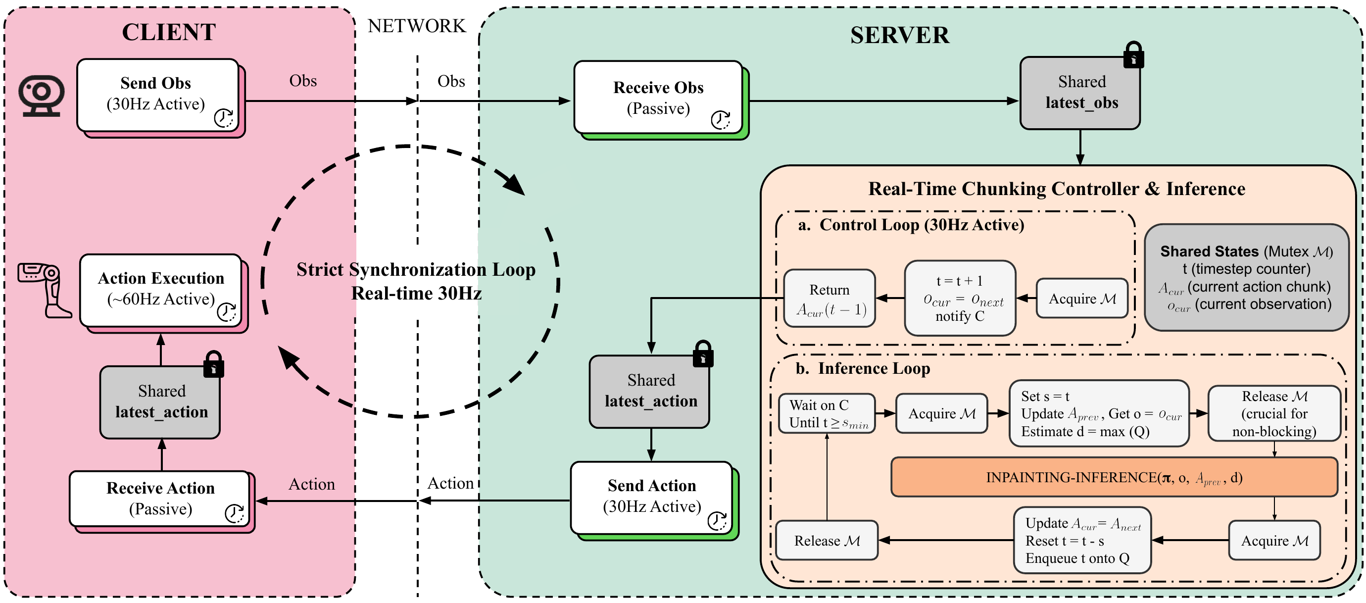
The solution: Two asynchronous threads
RTC splits inference into 2 threads running in parallel:
Policy thread (runs at ~6Hz, every 160ms):
- Receives the latest observation
- Runs full VLM + MM-DiT inference
- Outputs a chunk of 10 future actions (action_exec_horizon = 10)
- Updates the action buffer
Control thread (runs at 30-60Hz, every 16-33ms):
- Reads the next action from the buffer
- Sends it to System-0 (RL controller)
- If the buffer runs out of actions → uses the last action (hold)
Think of it this way: the policy thread is like a chef preparing 10 dishes at a time whenever they enter the kitchen, while the control thread is like a waiter continuously serving one dish at a time. The customer (robot) always has food (actions) available, even though the chef needs time to cook.
Timeline illustration
Time (ms):       0    33   66   99  132  165  198  231  264  297  330
                 |    |    |    |    |    |    |    |    |    |    |
Policy thread:   [====== Inference 1 =========]
                 → Outputs actions a1..a10
                                               [====== Inference 2 =========]
                                               → Outputs actions a11..a20

Control thread:  a1   a2   a3   a4   a5   a6   a7   a8   a9   a10  a11
                 ↑ Reads from buffer continuously at 30Hz ↑
Thanks to this overlap, the robot never has to wait. While inference 1 is running, the control thread continues executing actions from the previous inference. When inference 1 completes, the buffer is replenished with 10 new actions.
Training-time RTC: Teaching the model to accept "phase shifts"
There's a subtle problem: during training, each observation is perfectly aligned with the action at the same timestep. But during deployment with RTC, the observation may be a few steps older than the action currently being executed — because the policy thread takes 160ms to process, while the robot has already moved further.
Psi0 solves this with training-time masking: during training, for each training sample, it randomly masks out the first d tokens of the action sequence, where d ~ Uniform(0, d_max) and d_max = 6. This teaches the model "don't depend too heavily on the first d actions — they may have already been executed by the time you receive the observation."
# Training-time RTC masking
d = random.randint(0, d_max)  # d_max = 6
action_sequence = action_sequence[d:]  # Drop first d tokens
# Model learns to predict actions starting from position d
The result: the Psi0 model with RTC achieves 3-5% higher success rate compared to without RTC, and more importantly — significantly reduces collision rate because the robot responds more smoothly.

Results analysis: What can Psi0 actually do?
Results on 8 real-world tasks (Unitree G1)
| Task | Success Rate | Notes |
|---|---|---|
| Handoff object | 9/10 | Most stable — fewest subtasks |
| Place lunch box | 9/10 | Accurate navigation + placement |
| Pour from bottle | 8/10 | Requires precise tilt angle |
| Wipe bowl | 7/10 | Failures mainly due to cloth slipping |
| Fill water | 6/10 | Most difficult — requires bimanual coordination |
| Pull tray | 5/10 | Uneven pulling force → tray rotates |
| Stack cups | -- | Insufficient data reported |
| Arrange objects | -- | Insufficient data reported |
Failure mode analysis
Across 80 episodes (8 tasks x 10 episodes), the most common failure causes:
-
Grasp failure (35%): The robot doesn't grasp the object precisely — fingers slip or don't close with enough force. This is a limitation of the Dex3-1 gripper with 3 fingers, not a model error.
-
Navigation error (25%): The robot moves to the wrong position, especially when the worktable isn't at the standard location. The System-0 locomotion controller sometimes drifts.
-
Timing mismatch (20%): The robot releases the object too early or too late — action timing doesn't match the actual state. This is an inherent issue with open-loop action chunking.
-
Perception failure (20%): The VLM misidentifies objects, especially transparent ones (glass cups, water bottles) or under strong reflections.
Comparison with baselines
| Model | Avg Success Rate | Inference Time | Notes |
|---|---|---|---|
| Psi0 (RTC) | 73% | 160ms | Foundation model, staged training |
| Pi0.5 | 65% | 200ms | Co-training, larger model |
| GR00T N1.6 | 58% | 180ms | Naive DiT, NVIDIA |
| Diffusion Policy | 52% | 500ms | DDPM 100 steps, slow |
| H-RDT | 48% | 150ms | No VLM |
| EgoVLA | 45% | 250ms | Egocentric but no staged training |
| InternVLA-M1 | 42% | 300ms | General VLA, not robot-specific |
| ACT | 38% | 80ms | Fast but less accurate |
Psi0 leads thanks to the combination of staged training (avoiding negative transfer) and EgoDex pre-training (high-quality egocentric video data). Notably, ACT is the fastest but has the lowest accuracy — showing that model capacity matters more than inference speed when RTC is available.
Open-loop evaluation: Fast but not sufficient
If you want to quickly check a model without a simulator, open-loop evaluation is still useful for debugging:
# Open-loop evaluation pseudocode
for obs, gt_actions in test_dataset:
    pred_actions = model.predict(obs)

    # Compare predicted vs ground-truth
    l2_error = torch.norm(pred_actions - gt_actions, dim=-1).mean()

    # Cosine similarity for movement direction
    cos_sim = F.cosine_similarity(pred_actions, gt_actions, dim=-1).mean()

    print(f"L2 error: {l2_error:.4f}, Cosine sim: {cos_sim:.4f}")
However, always remember: low open-loop L2 error does not guarantee high closed-loop success rate. In the Psi0 paper, some baselines had lower open-loop error than Psi0 but failed more frequently in the simulator — because they weren't robust to compounding error.
A critical lesson for anyone working with VLA models: always evaluate with closed-loop; open-loop is only for sanity checks.
Pre-inference checklist
Here's a checklist to ensure you don't hit common errors:
- GPU: Need at least 1 GPU with 24GB VRAM (A5000/A100/H100). RTX 4090 also works but is slower.
- Docker: Docker installed with NVIDIA Container Toolkit for the SIMPLE simulator.
- Checkpoint: Fully downloaded (~4GB) and checksum verified.
- Port: Port 8000 not occupied by another service.
- Network: Server and SIMPLE container on the same network (use
--network host). - Disk space: At least 50GB free for Docker images + video recordings.
Summary
In this post, we walked through the complete Psi0 inference pipeline: from serving the model via HTTP, connecting the SIMPLE simulator for closed-loop evaluation, to detailed results analysis. Most importantly, Real-Time Chunking solves the latency problem elegantly — without sacrificing model capacity, without reducing control frequency, but by using 2 asynchronous threads + training-time masking so the robot responds smoothly.
In the next and final post of this series, we'll analyze ablation studies and extract the 5 most important lessons from Psi0 for anyone building foundation models for robots.
Related posts
- Diffusion Policy — Diffusion for robot control — The Flow Matching foundation that Psi0 improves upon
- VLA Models — When language meets action — Overview of Vision-Language-Action models
- Humanoid Loco-manipulation: Challenges and directions — The broader context of the problem Psi0 solves