The first three posts established a complete pipeline: live PlotJuggler stream from G1 (part 1), 23-joint layout with MCAP recording (part 2), and IMU analysis with FFT vibration detection (part 3).
But raw data is rarely enough for diagnosis. For example: /lowstate/motor_state[i]/tau gives you torque, /lowstate/motor_state[i]/dq gives you velocity — but mechanical power for that joint (τ × dq) doesn't exist in any channel. To find out which joint consumes the most energy during walking, you have to compute it yourself.
PlotJuggler solves this with the Custom Function Editor — a Lua scripting engine embedded in the GUI that lets you create new signal channels from existing ones, in real time.
Series Roadmap
| # | Post | Content |
|---|---|---|
| 1 | Setup & live connection | Install PlotJuggler, CycloneDDS, subscribe to /lowstate |
| 2 | 23-joint layout + MCAP | Multi-panel layout, MCAP files, phase portraits |
| 3 | IMU debug + FFT | Quaternion → Euler, FFT vibration, Moving Average foot_force |
| 4 | Lua Transforms (this post) | Custom Functions for power, tracking error, derived signals |
| 5 | ZMQ + video sim2real | ZMQ bridge from MuJoCo, camera overlay, sim vs real comparison |
Two Computation Methods in PlotJuggler
Before writing code, understand that PlotJuggler offers two mechanisms for computing derived signals with different use cases:
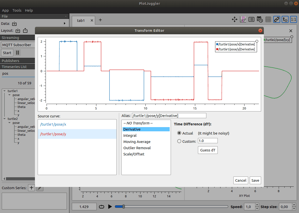
Method 1: Function Transform (Shift+T or "f(x)" icon on panel)
──────────────────────────────────────────────────────────────
  • Transforms 1 channel → 1 output channel (1-to-1)
  • For simple operations: abs(x), x * 180/pi, x[t] - x[t-1]
  • Cannot access other channels (only sees "current value" of dragged channel)
  • Result displays on the plot but is not saved to data tree

Method 2: Custom Function (Tools → Custom Functions → Add)
──────────────────────────────────────────────────────────
  • Write a Lua function receiving multiple input channels → 1 new output channel
  • Output channel appears in data tree, draggable into any panel
  • Function runs for each new timestamp (or during MCAP file replay)
  • Supports persistent global state (across calls) → compute integrals, rolling buffers
This post focuses on Custom Functions — powerful enough to compute per-joint power, tracking error, and any combined signal you need.
About the scripting language: PlotJuggler has always used Lua (via the sol2 library) for its Custom Function editor. The name "Lua Transforms" in this series reflects exactly that.
Opening the Custom Function Editor
From the PlotJuggler menu:
Tools → Custom Functions → Add new custom function
Or the shortcut Ctrl+Shift+C. The Function Editor window opens with two regions:
┌─────────────────────────────────────────────────────────┐
│  GLOBAL CODE (runs once on initialization)              │
│  ─ declare persistent variables, constants              │
├─────────────────────────────────────────────────────────┤
│  FUNCTION CODE (runs every timestamp)                   │
│  ─ receive input → return output                        │
├─────────────────────────────────────────────────────────┤
│  INPUT CHANNELS  │  OUTPUT CHANNEL NAME                 │
│  (drag from      │  (name of the new channel            │
│   data tree)     │   to create)                         │
└─────────────────────────────────────────────────────────┘
The Input Channels panel is critical — drag the /lowstate/... channels you want to compute from into this panel. The first channel becomes value in your Lua function; additional channels become v1, v2, etc.
The Custom Function API
PlotJuggler's Lua Custom Function is single-output: each function instance creates exactly one output channel. The function signature is:
-- Automatically wrapped by PlotJuggler:
function calc(time, value, v1, v2, ...)
  -- time  = current timestamp
  -- value = main input channel value
  -- v1    = first additional input channel value
  -- v2    = second additional input channel (if added)
  -- ...
  return some_number   -- this becomes the output channel value
end
Variables declared without local in Global Code are global and persist across calls.
Transform 1: Power Per Joint
The Problem
Each G1 joint has two channels:
tau— motor torque (N·m)dq— actual joint velocity (rad/s)
Mechanical power = τ × dq (W). Knowing which joint consumes the most power lets you:
- Detect abnormally high friction (joint friction → heat → bearing failure)
- Verify the controller is distributing load reasonably across joints
- Estimate battery drain in real time
Script Code
Create a new Custom Function for a specific joint (e.g., joint 10 — left hip):
1. Tools → Custom Functions → Add new custom function
2. Set output name: "power_hip_left"
3. Drag /lowstate/motor_state[10]/tau  into "main input"  (= value in the function)
4. Drag /lowstate/motor_state[10]/dq   into "additional source" (= v1 in the function)
Global Code (runs once):
-- No global variables needed for this transform
Function Code:
-- value = tau (N·m), v1 = dq (rad/s)
-- Mechanical power = τ × dq
return value * v1
Result: the power_hip_left channel appears in the data tree, displaying power (Watts) over time.
Repeat for the joints you suspect (typically knee + ankle on the same side to detect kinematic chain issues). For a quick debug session, you don't need all 23 — just 3–5 joints related to the observed abnormal behavior.
Drag the power_* channels into one panel, use View → Stacked Layout to view side by side. The joint with the highest spike when G1 climbs a step → that's the joint under the most load.
Transform 2: Total Mechanical Power
Since each Custom Function produces a single output, you have two approaches to sum across joints:
Option A (simple): After creating individual power_* channels, use the Built-in Add transform in PlotJuggler's Function Transforms to sum them. PlotJuggler's Sum(a, b) built-in handles this for a small number of signals.
Option B (one function, multiple inputs): Create one Custom Function that receives multiple tau/dq pairs as additional sources (v1..v5 for 3 joint pairs):
-- main = tau_hip_left, v1 = dq_hip_left
-- v2 = tau_knee_left,  v3 = dq_knee_left
-- v4 = tau_ankle_left, v5 = dq_ankle_left

local p_hip_L   = value * v1
local p_knee_L  = v2    * v3
local p_ankle_L = v4    * v5

local total = p_hip_L + p_knee_L + p_ankle_L

-- Exclude regenerative braking (negative) if only tracking power draw
if total < 0 then total = 0 end
return total
Why exclude negative values? When a motor brakes (velocity aligned with negative torque),
τ × dq < 0— the robot is regenerating energy. Keep negative values if you want to compute overall energy balance; clip to zero if you only care about when the robot is "drawing power."
Overlay the total power channel with IMU rpy[1] (pitch angle) to verify: when G1 leans forward more → does power increase correspondingly? If not → the controller is compensating incorrectly.
Transform 3: Velocity Tracking Error
The G1 controller sends a commanded velocity dq_d (desired) and the measured value is dq (actual). Tracking error reflects motor control quality and joint wear:
tracking_error_i = |dq_actual_i - dq_desired_i| / (|dq_desired_i| + ε)
dq is in /lowstate/motor_state[i]/dq. dq_d is in /lowstate/motor_state[i]/dq_d.
Create a Custom Function for joint 10 (left hip):
main input: /lowstate/motor_state[10]/dq   (dq_actual = value)
additional: /lowstate/motor_state[10]/dq_d (dq_desired = v1)
output name: "tracking_error_hip_left"
Global Code:
EPSILON = 0.001 -- avoid division by zero when robot is stationary (global, no 'local')
Function Code:
-- value = dq_actual (rad/s), v1 = dq_desired (rad/s)
local abs_error  = math.abs(value - v1)
local normalized = abs_error / (math.abs(v1) + EPSILON)
return normalized
How to read the results:
tracking_error > 0.5  → joint lagging heavily (>50% error)
                         Causes: high friction, worn joint, low controller gain
tracking_error ≈ 0    → perfect tracking (or robot stationary, dq_desired ≈ 0)
tracking_error > 2.0  → abnormal — inspect hardware
Saving and Loading Transform Templates
Scripts are lost when PlotJuggler closes. To reuse them:
Save script to .xml file:
In Custom Function Editor → "Save" button (floppy icon) → choose path
Example: ~/plotjuggler_scripts/g1_power_hip_left.xml
Load in a new session:
Tools → Custom Functions → Load from file → select .xml
Organize all G1 scripts in one directory with clear names:
~/plotjuggler_scripts/
  ├── g1_power_hip_left.xml
  ├── g1_power_knee_left.xml
  ├── g1_tracking_error_hip_left.xml
  └── g1_imu_quaternion_euler.xml   ← from part 3
When starting a new debug session, load all scripts → all derived channels appear immediately.
Case Study: Detecting an Overloaded Joint During Gait
A real-world scenario. Suppose G1 is performing a 30-second walking test, and you notice the robot starts limping slightly after 15 seconds.
Step 1: Replay the MCAP file from that session in PlotJuggler.
Step 2: Load g1_power_hip_left.xml, g1_power_knee_left.xml, and g1_tracking_error_hip_left.xml.
Step 3: Find the ~15 second timestamp and examine the comparison table:
Timestamp: t=14.8s → t=18.2s

Joint 10 (left hip):
  power_hip_left:          from 45W → 89W  (+98%)  ← ABNORMAL
  tracking_error_hip_left: from 0.12 → 0.67        ← tracking degrading

Joint 11 (left knee):
  power_knee_left:          from 38W → 92W  (+142%) ← VERY ABNORMAL
  tracking_error_knee_left: from 0.08 → 0.51

Joint 12 (left ankle):
  power_ankle_left:          stable ~15W
  tracking_error_ankle_left: stable ~0.09
Conclusion: The left hip + knee chain suddenly doubled in power and tracking error while the ankle remained normal → the problem is not at the end of the kinematic chain but in the middle. Check:
- Do joints 10/11 show elevated temperature? (log temperature if your G1 exposes this channel)
- Is there an unusual sound from joint 11?
- Overlay
tracking_error_hip_leftwithpower_hip_left— if tracking error increases before power increases → the motor is trying to compensate for increasing mechanical resistance.
Summary
The Custom Function Editor in PlotJuggler is not a replacement for Python/pandas — it's a real-time debug tool in the field. You don't need to write a new ROS node or export a new bag file when you want to see a new derived signal: write 2–5 lines of Lua in the Function Editor, drag the output channel into a panel, done.
The transforms in this post (joint_power, total power, tracking_error) are the foundation for any basic G1 debug session. Once comfortable, you can add:
energy_per_step— integrate power across one strideimpedance_estimate— estimate impedance from the tau/dq ratiogait_asymmetry— compare left vs right side power
The next post closes the series with the most advanced debug technique: ZMQ bridge from MuJoCo to PlotJuggler with synchronized camera feed for direct sim-to-real comparison.
Related Posts
- PlotJuggler + G1: IMU Debug Quaternion → Euler + FFT Vibration Analysis — Analyzing G1 IMU signals: quaternion to Euler, FFT resonance detection
- 23-Joint G1 Layout: MCAP Replay and Phase Portrait — Multi-panel organization, MCAP recording for offline replay
- ZMQ + VideoViewer: Sim-to-Real Debug with Camera Sync for G1 — ZMQ bridge from MuJoCo, camera overlay, sim vs real comparison