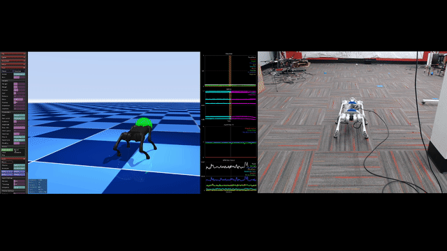
Why is Humanoid Control Difficult?
Humanoid robots have dozens of degrees of freedom (DOF) and must maintain balance on two legs while performing tasks with their arms. Compared to a fixed-base robot arm (6 DOF, no balance needed), humanoids are orders of magnitude more complex.
This article progresses from basics to advanced: Inverse Kinematics (IK) → Jacobian → Operational Space Control → Balance control (ZMP, CoM) → Task Prioritization. Each section includes Python code for hands-on practice.

Inverse Kinematics (IK) — The First Foundation
IK answers the question: "Given the desired position of an end-effector (hand, foot), find the corresponding joint angles."
Forward Kinematics (FK)
FK is the reverse process: given joint angles, calculate end-effector position. For a chain of joints, we use homogeneous transformations:
T_0_n = T_0_1 * T_1_2 * ... * T_(n-1)_n
Each T_i_(i+1) is a 4x4 matrix representing rotation and translation between two consecutive joints, typically using Denavit-Hartenberg (DH) parameters.
IK using Jacobian (Numerical)
With humanoid robots having 30+ DOF, analytical IK is very difficult (or impossible). The numerical method uses the Jacobian matrix:
import numpy as np
import mujoco

def compute_jacobian(model, data, body_id):
    """Compute Jacobian for one body in MuJoCo."""
    jacp = np.zeros((3, model.nv))  # position Jacobian
    jacr = np.zeros((3, model.nv))  # rotation Jacobian
    mujoco.mj_jacBody(model, data, jacp, jacr, body_id)
    return np.vstack([jacp, jacr])  # 6 x nv

def ik_step(model, data, body_id, target_pos, target_quat, step_size=0.5):
    """One IK step using damped least squares."""
    # Compute current position
    current_pos = data.xpos[body_id].copy()
    current_quat = data.xquat[body_id].copy()

    # Compute position error
    pos_error = target_pos - current_pos

    # Compute orientation error (using quaternion)
    quat_error = np.zeros(3)
    mujoco.mju_subQuat(quat_error, target_quat, current_quat)

    # Combine into 6D error
    error = np.concatenate([pos_error, quat_error])

    # Compute Jacobian
    J = compute_jacobian(model, data, body_id)

    # Damped least squares (Levenberg-Marquardt)
    damping = 1e-4
    JtJ = J.T @ J + damping * np.eye(model.nv)
    delta_q = np.linalg.solve(JtJ, J.T @ error)

    # Update joint positions
    data.qpos[:model.nv] += step_size * delta_q
    mujoco.mj_forward(model, data)

    return np.linalg.norm(error)

# Run IK loop
for i in range(100):
    err = ik_step(model, data, hand_body_id, target_pos, target_quat)
    if err < 1e-3:
        print(f"IK converged after {i+1} iterations")
        break
Damped Least Squares (or Levenberg-Marquardt) addresses the singularity problem — when Jacobian loses rank (robot at workspace boundary), Jacobian inversion becomes unstable. Adding damping lambda * I improves stability but reduces accuracy.
IK Libraries for Humanoid
- MuJoCo built-in:
mujoco.mj_jacBody()+ custom solver - Pink: IK library for Python, supports MuJoCo and Pinocchio
- Pinocchio: Rigid body dynamics library, IK + dynamics
- Drake: MIT/TRI toolbox, strong on optimization-based IK
Operational Space Control
IK only calculates desired position — but doesn't control force. In practice, humanoids need to control both position and force — this is Operational Space Control (Khatib, 1987).
Main Concept
Instead of controlling in joint space (q, dq, tau), we control in task space (x, dx, F):
F = Lambda * x_ddot_desired + mu + p
Where:
Lambda = (J * M^(-1) * J^T)^(-1)— task-space inertia matrixmu— Coriolis/centrifugal forces in task spacep— gravity forces in task spacex_ddot_desired— desired acceleration in task space
Convert back to joint torques:
tau = J^T * F + N^T * tau_null
Where N = I - J^T * Lambda * J * M^(-1) is the null-space projector — allows performing secondary tasks (e.g., maintaining balance) without affecting the primary task.
Operational Space Control Code
import numpy as np
import mujoco

class OperationalSpaceController:
    def __init__(self, model, data, body_id):
        self.model = model
        self.data = data
        self.body_id = body_id
        self.nv = model.nv

    def compute_task_space_control(self, x_des, dx_des, ddx_des, Kp, Kd):
        """Compute joint torques from task-space command."""
        m = self.model
        d = self.data

        # Mass matrix
        M = np.zeros((self.nv, self.nv))
        mujoco.mj_fullM(m, M, d.qM)

        # Jacobian
        J = compute_jacobian(m, d, self.body_id)[:3]  # Position only

        # Task-space inertia
        M_inv = np.linalg.inv(M)
        Lambda_inv = J @ M_inv @ J.T
        Lambda = np.linalg.inv(Lambda_inv)

        # Current task-space state
        x = d.xpos[self.body_id].copy()
        dx = J @ d.qvel

        # PD control in task space
        ddx_cmd = ddx_des + Kp * (x_des - x) + Kd * (dx_des - dx)

        # Task-space force
        F = Lambda @ ddx_cmd

        # Coriolis compensation
        bias = d.qfrc_bias.copy()  # C(q,dq)*dq + g(q)
        mu_p = J @ M_inv @ bias
        F += mu_p

        # Map to joint torques
        tau = J.T @ F

        # Null-space: maintain default posture
        N = np.eye(self.nv) - J.T @ Lambda @ J @ M_inv
        q_default = np.zeros(self.nv)
        tau_null = 10.0 * (q_default - d.qpos[:self.nv]) - 2.0 * d.qvel
        tau += N.T @ tau_null

        return tau
Balance Control — ZMP and CoM
Humanoids must maintain balance while performing tasks. Two key concepts:
Center of Mass (CoM)
CoM is the center of mass of the entire robot. For the robot not to fall, the projection of CoM onto the ground must lie within the support polygon (the region created by foot contact points).
Zero Moment Point (ZMP)
ZMP is the point on the ground where the sum of all moments (gravity + inertial) equals zero. Balance condition:
ZMP lies within support polygon
When ZMP approaches the support polygon boundary, the robot is about to fall. The controller must adjust to pull ZMP back to center.

ZMP Computation Code
def compute_zmp(model, data):
    """Compute ZMP from MuJoCo simulation data."""
    # Total mass
    total_mass = sum(model.body_mass)

    # CoM position and acceleration
    com_pos = np.zeros(3)
    com_acc = np.zeros(3)

    for i in range(model.nbody):
        m_i = model.body_mass[i]
        com_pos += m_i * data.xipos[i]
        # Acceleration from applied forces
        com_acc += data.xfrc_applied[i, :3]  # Simplified

    com_pos /= total_mass
    com_acc /= total_mass

    g = 9.81
    # ZMP formula
    zmp_x = com_pos[0] - com_pos[2] * com_acc[0] / (g + com_acc[2])
    zmp_y = com_pos[1] - com_pos[2] * com_acc[1] / (g + com_acc[2])

    return np.array([zmp_x, zmp_y])

def compute_support_polygon(contact_positions):
    """Compute support polygon from contact points."""
    from scipy.spatial import ConvexHull
    if len(contact_positions) < 3:
        return contact_positions
    points_2d = contact_positions[:, :2]  # Only x, y
    hull = ConvexHull(points_2d)
    return points_2d[hull.vertices]
Linear Inverted Pendulum Model (LIPM)
For simplification, humanoids are often modeled as a linear inverted pendulum (LIPM):
ddot_x_com = (g / z_com) * (x_com - x_zmp)
From this, we design a controller to adjust x_zmp so x_com follows the desired trajectory. This is the foundation of ZMP-based walking — the most classical walking approach for humanoids.
Task Prioritization — Doing Multiple Things at Once
Humanoids need to perform multiple tasks simultaneously: maintain balance (highest priority), move (medium priority), manipulate with arms (lower priority). Task prioritization solves this.
Null-Space Projection
Idea: lower-priority tasks are projected into the null space of higher-priority tasks — meaning lower-priority tasks execute only if they don't affect higher priorities.
def prioritized_control(tasks, model, data):
    """
    tasks = [(J1, F1), (J2, F2), ...] in order of decreasing priority.
    """
    nv = model.nv
    tau = np.zeros(nv)
    N = np.eye(nv)  # Null-space projector

    for J_i, F_i in tasks:
        # Project task into null space of previous tasks
        J_bar = J_i @ N

        # Pseudoinverse
        J_bar_pinv = np.linalg.pinv(J_bar)

        # Torque for this task
        tau += N @ J_bar_pinv @ F_i

        # Update null space
        N = N @ (np.eye(nv) - J_bar_pinv @ J_bar)

    return tau

# Usage:
# Task 1 (highest): Maintain balance (CoM control)
# Task 2: Move feet
# Task 3: Manipulate with hands
# Task 4 (lowest): Maintain default posture
tasks = [
    (J_com, F_balance),
    (J_feet, F_locomotion),
    (J_hand, F_manipulation),
    (J_posture, F_posture)
]
tau = prioritized_control(tasks, model, data)
Whole-Body QP Controller
In practice, many modern systems use Quadratic Programming (QP) instead of null-space projection:
minimize: ||J_task * ddq - ddx_desired||^2 + w * ||tau||^2
subject to:
    M * ddq + C * dq + g = S * tau + J_c^T * f_c   (dynamics)
    f_c in friction cone                            (no slip)
    tau_min <= tau <= tau_max                       (actuator limits)
    ZMP in support polygon                          (balance)
QP naturally handles constraints (torque limits, friction cone, balance) — something null-space projection cannot.
Popular libraries: qpOASES, OSQP, Pinocchio + ProxQP.
Control Pipeline Summary
Task Planner (manipulate, move, ...)
    |
    v
Task-Space Controller (Operational Space / QP)
    |
    v
Balance Controller (ZMP / CoM tracking)
    |
    v
Whole-Body IK / ID (Jacobian, dynamics)
    |
    v
Joint Torque Commands → Actuators
Each layer solves a different problem, from high-level planning to low-level torque control. In the next article, we'll dive into Model Predictive Control (MPC) — a more powerful method for real-time whole-body humanoid control.

Next in This Series
- Part 1: Humanoid Robots 2026: Complete Platform Overview
- Part 3: Whole-Body MPC: Real-time Full-Body Control — MPC with MuJoCo, iLQR
- Part 4: RL for Humanoid: From Humanoid-Gym to Sim2Real
Related Articles
- Inverse Kinematics for 6-DOF Robots — Detailed IK for robot arms
- RL for Bipedal Walking — RL approach for balance and locomotion
- MoveIt 2 Motion Planning — Motion planning with ROS 2
- Simulation for Robotics — Choosing the right simulator