Inverse Kinematics là gì và tại sao quan trọng?
Inverse Kinematics (IK) cho robot arm 6 bậc tự do là bài toán cốt lõi trong robotics: cho vị trí và hướng mong muốn của end-effector, tìm bộ góc khớp (joint angles) tương ứng. Nếu bạn từng lập trình robot gắp vật, bạn biết rằng con người nghĩ theo tọa độ Cartesian ("đưa tay đến điểm x, y, z") nhưng robot cần góc từng khớp. IK chính là cầu nối giữa hai thế giới đó.
Bài viết này sẽ đi từ lý thuyết Denavit-Hartenberg (DH), qua forward kinematics, đến numerical IK solver hoàn chỉnh bằng Python. Code chạy được ngay với NumPy — không cần thư viện robotics chuyên dụng.

Denavit-Hartenberg Convention
Tại sao cần DH Parameters?
Mỗi robot arm có cấu hình khớp (joint) và link khác nhau. DH convention cung cấp một phương pháp chuẩn hóa để mô tả mối quan hệ hình học giữa các khớp liên tiếp bằng đúng 4 tham số cho mỗi khớp:
| Tham số | Ký hiệu | Ý nghĩa |
|---|---|---|
| Link length | a_i | Khoảng cách giữa trục z_{i-1} và z_i dọc theo trục x_i |
| Link twist | alpha_i | Góc xoay từ z_{i-1} đến z_i quanh trục x_i |
| Link offset | d_i | Khoảng cách dọc theo trục z_{i-1} |
| Joint angle | theta_i | Góc xoay quanh trục z_{i-1} (biến khớp cho revolute joint) |
Ma trận biến đổi DH
Mỗi bộ DH parameters cho ra một homogeneous transformation matrix 4x4:
import numpy as np

def dh_matrix(theta, d, a, alpha):
    """
    Tạo ma trận biến đổi DH 4x4.
    theta: góc khớp (rad)
    d: link offset
    a: link length
    alpha: link twist (rad)
    """
    ct, st = np.cos(theta), np.sin(theta)
    ca, sa = np.cos(alpha), np.sin(alpha)

    return np.array([
        [ct, -st * ca,  st * sa, a * ct],
        [st,  ct * ca, -ct * sa, a * st],
        [0,   sa,       ca,      d     ],
        [0,   0,        0,       1     ]
    ])
Ma trận này encode cả rotation lẫn translation. Nhân chuỗi 6 ma trận lại ta được forward kinematics — vị trí và hướng của end-effector từ bộ góc khớp.
Forward Kinematics cho robot 6-DOF
Ví dụ: Robot dạng Puma 560
Dưới đây là bảng DH parameters mẫu cho robot 6 khớp revolute (đơn vị: mét, radian):
# DH Parameters cho robot 6-DOF dạng anthropomorphic
# Mỗi hàng: [a, alpha, d, theta_offset]
# theta thực tế = theta_variable + theta_offset
DH_PARAMS = [
    # a      alpha        d      theta_offset
    [0.0,    np.pi/2,     0.4,   0.0],   # Joint 1 (base rotation)
    [0.25,   0.0,         0.0,   0.0],   # Joint 2 (shoulder)
    [0.025,  np.pi/2,     0.0,   0.0],   # Joint 3 (elbow)
    [0.0,   -np.pi/2,     0.28,  0.0],   # Joint 4 (wrist roll)
    [0.0,    np.pi/2,     0.0,   0.0],   # Joint 5 (wrist pitch)
    [0.0,    0.0,         0.1,   0.0],   # Joint 6 (wrist yaw)
]

def forward_kinematics(joint_angles, dh_params=DH_PARAMS):
    """
    Tính vị trí và hướng end-effector từ góc khớp.
    Trả về ma trận 4x4 (rotation + position).
    """
    T = np.eye(4)
    for i, (a, alpha, d, offset) in enumerate(dh_params):
        theta = joint_angles[i] + offset
        T = T @ dh_matrix(theta, d, a, alpha)
    return T

# Test: tất cả khớp ở vị trí 0
q_home = np.zeros(6)
T_home = forward_kinematics(q_home)
position = T_home[:3, 3]
print(f"Home position: x={position[0]:.3f}, y={position[1]:.3f}, z={position[2]:.3f}")
Trích xuất Position và Orientation
def extract_pose(T):
    """Trích xuất position (xyz) và rotation matrix từ T 4x4."""
    position = T[:3, 3]
    rotation = T[:3, :3]
    return position, rotation

def rotation_to_euler(R):
    """Chuyển rotation matrix sang Euler angles (ZYX convention)."""
    sy = np.sqrt(R[0, 0]**2 + R[1, 0]**2)
    singular = sy < 1e-6

    if not singular:
        roll  = np.arctan2(R[2, 1], R[2, 2])
        pitch = np.arctan2(-R[2, 0], sy)
        yaw   = np.arctan2(R[1, 0], R[0, 0])
    else:
        roll  = np.arctan2(-R[1, 2], R[1, 1])
        pitch = np.arctan2(-R[2, 0], sy)
        yaw   = 0.0

    return np.array([roll, pitch, yaw])
Jacobian Matrix — Chìa khóa của Numerical IK
Jacobian là gì?
Jacobian matrix J mô tả mối quan hệ vi phân giữa vận tốc khớp và vận tốc end-effector:
v = J(q) * dq
Trong đó v là vector 6D (3 linear + 3 angular velocity), q là vector góc khớp. Đối với numerical IK, Jacobian cho phép ta tính: "nếu muốn end-effector dịch chuyển delta_x, cần thay đổi góc khớp bao nhiêu?"
Tính Jacobian bằng phương pháp số
Cách đơn giản và robust nhất là finite differences:
def compute_jacobian(joint_angles, dh_params=DH_PARAMS, delta=1e-6):
    """
    Tính numerical Jacobian (6x6) bằng finite differences.
    Hàng 0-2: linear velocity (dx, dy, dz)
    Hàng 3-5: angular velocity (drx, dry, drz)
    """
    n_joints = len(joint_angles)
    J = np.zeros((6, n_joints))

    T_current = forward_kinematics(joint_angles, dh_params)
    pos_current, R_current = extract_pose(T_current)
    euler_current = rotation_to_euler(R_current)

    for i in range(n_joints):
        q_perturbed = joint_angles.copy()
        q_perturbed[i] += delta

        T_perturbed = forward_kinematics(q_perturbed, dh_params)
        pos_perturbed, R_perturbed = extract_pose(T_perturbed)
        euler_perturbed = rotation_to_euler(R_perturbed)

        # Linear velocity columns
        J[:3, i] = (pos_perturbed - pos_current) / delta
        # Angular velocity columns
        J[3:, i] = (euler_perturbed - euler_current) / delta

    return J

Numerical IK Solver: Newton-Raphson
Thuật toán
Ý tưởng cốt lõi: lặp đi lặp lại việc tính error giữa pose hiện tại và pose mong muốn, rồi dùng pseudo-inverse Jacobian để cập nhật góc khớp.
while |error| > tolerance:
    error = target_pose - current_pose
    dq = J_pinv * error
    q = q + dq
Implementation đầy đủ
def pose_error(T_current, T_target):
    """
    Tính error 6D giữa pose hiện tại và target.
    Returns: [dx, dy, dz, drx, dry, drz]
    """
    pos_err = T_target[:3, 3] - T_current[:3, 3]

    R_current = T_current[:3, :3]
    R_target = T_target[:3, :3]
    R_err = R_target @ R_current.T

    # Trích xuất rotation error dạng axis-angle
    angle = np.arccos(np.clip((np.trace(R_err) - 1) / 2, -1, 1))
    if angle < 1e-6:
        rot_err = np.zeros(3)
    else:
        rot_err = angle / (2 * np.sin(angle)) * np.array([
            R_err[2, 1] - R_err[1, 2],
            R_err[0, 2] - R_err[2, 0],
            R_err[1, 0] - R_err[0, 1]
        ])

    return np.concatenate([pos_err, rot_err])


def inverse_kinematics(T_target, q_init=None, dh_params=DH_PARAMS,
                        max_iter=200, pos_tol=1e-4, rot_tol=1e-3,
                        damping=0.1):
    """
    Numerical IK solver dùng Damped Least Squares (Levenberg-Marquardt).

    Args:
        T_target: ma trận 4x4 mục tiêu
        q_init: góc khớp khởi tạo (None = zeros)
        max_iter: số vòng lặp tối đa
        pos_tol: sai số vị trí chấp nhận (mét)
        rot_tol: sai số góc chấp nhận (rad)
        damping: hệ số damping lambda (tránh singularity)

    Returns:
        q_solution: bộ góc khớp nghiệm
        success: True nếu hội tụ
        iterations: số vòng lặp thực tế
    """
    n_joints = len(dh_params)
    q = q_init.copy() if q_init is not None else np.zeros(n_joints)

    for iteration in range(max_iter):
        T_current = forward_kinematics(q, dh_params)
        error = pose_error(T_current, T_target)

        pos_err_norm = np.linalg.norm(error[:3])
        rot_err_norm = np.linalg.norm(error[3:])

        # Kiểm tra hội tụ
        if pos_err_norm < pos_tol and rot_err_norm < rot_tol:
            return q, True, iteration

        # Tính Jacobian và pseudo-inverse có damping
        J = compute_jacobian(q, dh_params)
        # Damped Least Squares: dq = J^T (J J^T + lambda^2 I)^(-1) * error
        JJT = J @ J.T
        dq = J.T @ np.linalg.solve(
            JJT + damping**2 * np.eye(6), error
        )

        q = q + dq

        # Giới hạn góc khớp trong [-pi, pi]
        q = np.mod(q + np.pi, 2 * np.pi) - np.pi

    return q, False, max_iter


# === VÍ DỤ SỬ DỤNG ===

# Bước 1: Forward kinematics để tạo target pose
q_desired = np.array([0.3, -0.5, 0.8, 0.1, -0.3, 0.6])
T_target = forward_kinematics(q_desired)

print("Target position:", T_target[:3, 3])
print("Target angles (ground truth):", np.degrees(q_desired))

# Bước 2: Giải IK từ initial guess khác
q_init = np.array([0.0, 0.0, 0.0, 0.0, 0.0, 0.0])
q_solution, success, iters = inverse_kinematics(T_target, q_init)

print(f"\nIK {'converged' if success else 'FAILED'} after {iters} iterations")
print(f"Solution angles: {np.degrees(q_solution).round(2)}")

# Verify
T_result = forward_kinematics(q_solution)
pos_error = np.linalg.norm(T_target[:3, 3] - T_result[:3, 3])
print(f"Position error: {pos_error*1000:.3f} mm")
Damped Least Squares vs Pure Pseudo-Inverse
Vấn đề Singularity
Khi robot gần singularity (ví dụ: hai khớp wrist thẳng hàng), Jacobian gần như singular, pseudo-inverse cho ra giá trị cực lớn khiến robot "bay" không kiểm soát.
Damped Least Squares (còn gọi là Levenberg-Marquardt) thêm hệ số damping lambda:
dq = J^T (J J^T + lambda^2 I)^(-1) * error
Khi lambda = 0, ta có pseudo-inverse thuần. Khi lambda lớn, chuyển động chậm hơn nhưng ổn định gần singularity. Trong thực tế, lambda = 0.01 - 0.5 hoạt động tốt cho hầu hết robot.
Adaptive Damping
Một kỹ thuật nâng cao là điều chỉnh lambda theo khoảng cách đến singularity:
def adaptive_damping(J, lambda_min=0.01, lambda_max=0.5):
    """Tăng damping khi gần singularity."""
    # Manipulability measure
    w = np.sqrt(max(np.linalg.det(J @ J.T), 0))
    # Threshold
    w_threshold = 0.05
    if w < w_threshold:
        ratio = 1.0 - (w / w_threshold)**2
        return lambda_min + ratio * (lambda_max - lambda_min)
    return lambda_min
Mẹo thực tế khi implement IK
1. Multiple Solutions
Robot 6-DOF thường có tối đa 8 nghiệm cho cùng một target pose. Initial guess quyết định bạn nhận được nghiệm nào. Trong ứng dụng thực tế, chọn nghiệm gần cấu hình hiện tại nhất để giảm chuyển động:
def best_ik_solution(T_target, q_current, n_trials=10):
    """Thử nhiều initial guess, chọn nghiệm gần nhất."""
    best_q = None
    best_dist = float('inf')

    for _ in range(n_trials):
        q_init = q_current + np.random.uniform(-0.5, 0.5, 6)
        q_sol, success, _ = inverse_kinematics(T_target, q_init)
        if success:
            dist = np.linalg.norm(q_sol - q_current)
            if dist < best_dist:
                best_dist = dist
                best_q = q_sol

    return best_q
2. Joint Limits
Robot thật có giới hạn góc khớp. Thêm clamping sau mỗi iteration:
JOINT_LIMITS = [
    (-np.pi, np.pi),       # Joint 1
    (-np.pi/2, np.pi/2),   # Joint 2
    (-np.pi*3/4, np.pi*3/4), # Joint 3
    (-np.pi, np.pi),       # Joint 4
    (-np.pi/2, np.pi/2),   # Joint 5
    (-np.pi, np.pi),       # Joint 6
]

def clamp_joints(q, limits=JOINT_LIMITS):
    return np.array([
        np.clip(q[i], limits[i][0], limits[i][1])
        for i in range(len(q))
    ])
3. Workspace Check
Trước khi chạy IK, kiểm tra target có nằm trong workspace:
def in_workspace(T_target, dh_params=DH_PARAMS):
    """Kiểm tra nhanh target có trong tầm với không."""
    pos = T_target[:3, 3]
    dist = np.linalg.norm(pos)
    # Tổng chiều dài tất cả links
    max_reach = sum(
        np.sqrt(p[0]**2 + p[2]**2) for p in dh_params
    )
    return dist <= max_reach * 0.95  # 95% safety margin
Visualization với Matplotlib
import matplotlib.pyplot as plt
from mpl_toolkits.mplot3d import Axes3D

def plot_robot(joint_angles, dh_params=DH_PARAMS, ax=None):
    """Vẽ robot arm 3D từ bộ góc khớp."""
    if ax is None:
        fig = plt.figure(figsize=(10, 8))
        ax = fig.add_subplot(111, projection='3d')

    positions = [np.array([0, 0, 0])]
    T = np.eye(4)

    for i, (a, alpha, d, offset) in enumerate(dh_params):
        theta = joint_angles[i] + offset
        T = T @ dh_matrix(theta, d, a, alpha)
        positions.append(T[:3, 3].copy())

    positions = np.array(positions)
    ax.plot(positions[:, 0], positions[:, 1], positions[:, 2],
            'o-', linewidth=3, markersize=8, color='steelblue')
    ax.scatter(*positions[-1], color='red', s=100, zorder=5,
               label='End-effector')
    ax.scatter(*positions[0], color='green', s=100, zorder=5,
               label='Base')

    ax.set_xlabel('X (m)')
    ax.set_ylabel('Y (m)')
    ax.set_zlabel('Z (m)')
    ax.legend()
    ax.set_title('Robot Arm Configuration')
    plt.tight_layout()
    return ax

# Vẽ cấu hình home và cấu hình IK solution
fig, (ax1, ax2) = plt.subplots(1, 2, figsize=(16, 7),
                                subplot_kw={'projection': '3d'})
plot_robot(np.zeros(6), ax=ax1)
ax1.set_title('Home Configuration')

plot_robot(q_solution, ax=ax2)
ax2.set_title('IK Solution')
plt.savefig('robot_ik_comparison.png', dpi=150)
plt.show()

Bước tiếp theo
Code trong bài viết này là self-contained — chỉ cần NumPy và Matplotlib. Bạn có thể mở rộng thêm:
- Trajectory planning: Nội suy giữa nhiều điểm IK bằng cubic spline
- Collision avoidance: Tích hợp với MoveIt2 trong ROS 2
- Real-time control: Gửi góc khớp qua Serial/CAN bus đến motor driver
Nếu bạn mới bắt đầu với Python cho robotics, hãy đọc bài Lập trình điều khiển robot với Python để nắm nền tảng GPIO, PID, và computer vision.