Ψ₀ Hands-On (2): The Three-Tier Architecture — Brain, Hands, and Legs of the Robot
In the previous article, we understood the big picture of Ψ₀ and why it matters. Now it is time to pop the hood and see what is inside. This article takes a deep dive into the three-tier architecture — how each component works, how data flows through the system, and why each design decision was made.
Fair warning: this article is technically dense. But I will do my best to keep everything as intuitive as possible.
The Big Picture: Data Flow
Before diving into each system, let us look at the entire pipeline from end to end. When the robot receives a command ("pick up the glass of water"), here is what happens:
Camera (320x240 RGB)
    │
    ▼
System-2: Qwen3-VL-2B (VLM)
    │ → Visual features + Text features
    ▼
System-1: MM-DiT (~500M params)
    │ → Action chunks (28 DoF upper body + 8 locomotion commands)
    ├── 28 DoF → Directly to arm + hand motors
    ▼
System-0: AMO RL Controller
    │ ← 8 DoF commands (velocity, heading, height...)
    ▼
15 DoF legs → Leg motors
The entire pipeline runs with a latency of approximately 160ms — fast enough for real-time control. Now let us zoom into each system.
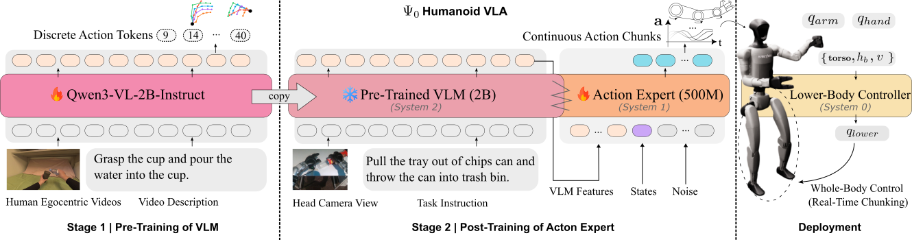
System-2: The Brain That Sees and Understands — Qwen3-VL-2B
Why Qwen3-VL-2B?
System-2 is a Vision-Language Model (VLM) whose job is to take images from the camera and text commands, then extract meaningful features for System-1 to use. The research team chose Qwen3-VL-2B — the 2-billion parameter version of Qwen3-VL from Alibaba — for three reasons:
-
Right-sized: 2B parameters is powerful enough to understand complex images, yet small enough to run in real-time on an edge GPU. Larger models like LLaVA-13B or Qwen-VL-7B would be too slow for robot control at 160ms latency.
-
Strong vision performance: Qwen3-VL is one of the best small VLMs for visual understanding, particularly in recognizing objects and understanding 3D spatial relationships from 2D images.
-
Pre-trained out of the box: The model has already been trained on billions of image-text pairs, so it comes with built-in ability to recognize everyday objects (cups, bottles, boxes, door handles...) that robots need to interact with.

How It Works
System-2 takes as input:
- An RGB image at 320x240 pixels from the camera mounted on the robot's head (egocentric view)
- A text instruction — a natural language command, e.g., "pick up the red cup"
And outputs visual-language features — a tensor containing semantic information about both the image and text, which is passed into System-1.
# Simplified pseudo-code
image = camera.capture()  # 320x240x3 RGB
text = "pick up the red cup"

# VLM processing
visual_tokens = qwen3_vision_encoder(image)   # [N, D]
text_tokens = qwen3_text_encoder(text)        # [M, D]
features = qwen3_cross_attention(visual_tokens, text_tokens)  # [N+M, D]
One important detail: System-2 is completely frozen during Ψ₀ training. This means the research team does not fine-tune the VLM — they use the pre-trained model as-is. This has two implications:
- Advantage: Significant savings in training resources. No need to compute gradients through 2B parameters.
- Potential drawback: The VLM may not be optimally adapted for the specific domain (robot egocentric view). However, experiments show that Qwen3-VL is good enough.
If you want a deeper understanding of how VLA models generally use VLMs, read our article on VLA models in the AI for Robots series.
System-1: The Acting Hands — MM-DiT Action Expert
This is the heart of Ψ₀. System-1 is an action expert with approximately 500 million parameters, responsible for generating sequences of actions (action chunks) from System-2's features. It is built on three key technologies: MM-DiT, Flow Matching, and Action Chunking.
MM-DiT: Why Not Use a Standard DiT?
DiT (Diffusion Transformer) is a transformer architecture designed for diffusion models. But Ψ₀ uses a variant called MM-DiT (Multi-Modal DiT), inspired by the architecture in Stable Diffusion 3. The difference lies in two critical aspects:
1. Separate Modulation
In a standard DiT (Naive DiT), all modalities (image, text, action) pass through the same set of modulation parameters. This means the model uses a shared way to "adjust" processing for every type of input.
MM-DiT changes this: each modality has its own modulation parameters. Specifically:
- Visual features from the VLM get their own modulation parameters
- Action tokens get their own modulation parameters
- Timestep embeddings get their own modulation parameters
Why does this matter? Because visual features and action tokens are fundamentally different in nature. Visual features represent static spatial information (object positions, shapes). Action tokens represent dynamic temporal sequences (robot joint positions over time). Forcing them through the same "filter" loses information.
2. Joint Attention
Despite separate modulation, MM-DiT still allows joint attention across modalities. This means action tokens can "look at" visual features during attention computation, and vice versa.
# Simplified MM-DiT block
class MMDiTBlock:
    def forward(self, visual_tokens, action_tokens, timestep):
        # Separate modulation
        v_scale, v_shift = self.visual_modulation(timestep)
        a_scale, a_shift = self.action_modulation(timestep)

        visual_tokens = v_scale * self.norm(visual_tokens) + v_shift
        action_tokens = a_scale * self.norm(action_tokens) + a_shift

        # Joint attention - both modalities attend to each other
        all_tokens = concat(visual_tokens, action_tokens)
        all_tokens = self.joint_attention(all_tokens)

        # Split back
        visual_tokens, action_tokens = split(all_tokens)
        return visual_tokens, action_tokens
The combination of separate modulation + joint attention creates the best balance: each modality is processed in a way that suits its nature, while still being able to exchange information with the other modality.
Flow Matching: From Noise to Action
This is the most important mathematical component in Ψ₀. But do not worry — I will explain it intuitively first, then introduce the formulas.
The Intuitive Idea
Imagine you are standing in the middle of a foggy field (noise). You want to reach a specific house (the correct action). Flow Matching gives you a compass — at every point in the field, the compass tells you which direction to go. If you follow the compass long enough, you will reach the house.
Mathematically, this "compass" is a velocity field v(x, tau) — at every point x in action space and every time step tau, it tells you which direction to move.
The Core Formula
Flow Matching defines a straight-line path from noise to action:
x(tau) = (1 - tau) * epsilon + tau * a
Where:
- epsilon is Gaussian noise (a random starting point)
- a is the ground-truth action (the destination)
- tau is in [0, 1] — tau=0 is pure noise, tau=1 is the complete action
The corresponding velocity field is:
v*(x, tau) = a - epsilon
Surprisingly simple — the velocity field is just the direction from noise to action. The model is trained to predict this velocity field:
Loss = || v_theta(x(tau), tau, c) - (a - epsilon) ||^2
Where c is the conditioning (visual features from System-2), and v_theta is the MM-DiT model with parameters theta.

Flow Matching vs. DDPM Diffusion
If you have read about Diffusion Policy, you will notice that Flow Matching differs from DDPM in several key ways:
| Flow Matching | DDPM Diffusion | |
|---|---|---|
| Path | Straight (linear interpolation) | Curved (Markov chain) |
| Inference steps | Few (1-10 steps) | Many (50-1000 steps) |
| Speed | Much faster | Slow |
| Training stability | More stable | Can be unstable |
| Quality | Comparable or better | Good |
Ψ₀ uses 10 denoising steps during inference. At each step, the model takes the current state x(tau), predicts the velocity v, and updates: x(tau + delta_tau) = x(tau) + delta_tau * v. After 10 steps, pure noise becomes a complete action.
Action Chunking: Predicting the Future
Instead of predicting one action at a time, System-1 predicts a chunk of H consecutive actions simultaneously. In Ψ₀, H is typically 16-32 timesteps (equivalent to 0.8-1.6 seconds at 20Hz).
Why is chunking important?
-
Temporal coherence: When predicting individual actions, consecutive actions can "jitter" — one timestep tells the arm to go right, the next tells it to go left. Predicting an entire chunk ensures a smooth action sequence.
-
Handling latency: The robot needs approximately 160ms for one inference pass. If it only predicted 1 action, the robot would "freeze" for 160ms between each action. With chunking, the robot can execute previously predicted actions while the model computes the next batch.
-
Long-horizon understanding: Predicting 16 steps into the future requires the model to grasp a longer-term "plan," not just immediate reflexes.
FAST Tokenizer: Compressing Actions into Tokens
An important technical detail: before feeding actions into the MM-DiT, Ψ₀ uses the FAST tokenizer to encode continuous actions into discrete tokens. FAST (Fast Action Sequence Tokenizer) compresses action sequences into a compact representation by:
- Quantizing joint angle values
- Grouping highly correlated DoFs
- Significantly reducing data dimensionality
This allows the MM-DiT to process actions like "language" — each action token is equivalent to a "word" describing a movement. After inference, the output tokens are decoded back into continuous joint angle values.
System-0: The Autonomous Legs — AMO RL Controller
System-0 is the "balance keeper" of Ψ₀. It is an RL policy (a policy trained via Reinforcement Learning) called AMO (Agile Mobility Oracle), responsible for controlling the robot's legs.
Input/Output
-
Input (8 DoF commands): From System-1, including:
- Translational velocity x, y (forward/backward, left/right)
- Rotational velocity (yaw rate)
- Body height
- Body tilt angles (pitch, roll)
- Stepping frequency
- Step height
- Stance/swing ratio
-
Output (15 DoF): Direct commands to 15 motors in both legs (each leg: 3-DoF hip, 1-DoF knee, 2-DoF ankle, plus auxiliary DoFs).
Why RL Instead of a Learned Policy?
Bipedal locomotion is a problem that RL has already solved very well. Training an RL policy for walking and balancing in simulation (Isaac Gym, MuJoCo) and then performing sim-to-real transfer has become an industry standard — Unitree is one of the companies doing this best.
Since RL policies for locomotion are already very mature, there is no reason to retrain them end-to-end alongside manipulation. Keeping System-0 separate has several advantages:
- Robustness: The RL policy has been tested over millions of steps in simulation and is very stable.
- Safety: If System-1 generates unusual actions for the upper body, System-0 still prevents the robot from falling.
- Modularity: You can swap System-0 with a different policy without affecting System-1.
If you are not yet clear on how RL is used in humanoid locomotion, check out our article on RL for humanoids in the Humanoid Robot Engineering series.
Action Space: 43 DoF and How It Changes Across Stages
A subtle but important point: Ψ₀'s action space changes between training stages. This is not an oversight — it is a deliberate design choice.
Pre-training: 48-DoF Task Space
During the pre-training stage on egocentric video (EgoDex), the model predicts actions in task space — that is, the position and orientation of the hands in 3D space. Specifically:
- Each hand: 6-DoF pose (3 position xyz + 3 orientation rpy) = 12
- Each finger (simplified): Bend angles = ~12 per hand x 2 = 24
- Total: ~48 DoF in task space
Why use task space for pre-training? Because human video data only tells us where the hand is (via hand tracking), not the specific robot joint angles. Task space is a shared representation between humans and robots.
Post-training & Fine-tuning: 36-DoF Joint Space
When switching to real robot data (Stages 2 and 3), the model transitions to joint space — directly controlling the angle of each joint:
- 2 arms x 7-DoF = 14 DoF
- 2 Dex3-1 hands x 7-DoF = 14 DoF
- 8 locomotion commands for System-0
- Total: 36 DoF output from System-1
The transition from task space to joint space is a crucial step — it allows the model to "translate" general knowledge from human video into specific control commands for the Unitree G1 robot.
The Full 43-DoF
The total 43 DoF across the robot = 28 upper-body DoF (directly from System-1) + 15 leg DoF (from System-0, receiving 8 commands from System-1):
System-1 Output:
├── 7-DoF left arm      ─────────── Direct → Motor
├── 7-DoF right arm     ─────────── Direct → Motor
├── 7-DoF left hand     ─────────── Direct → Motor
├── 7-DoF right hand    ─────────── Direct → Motor
└── 8-DoF locomotion cmd   ──┐
                              │
System-0 (AMO RL):            │
├── Input: 8-DoF commands  ◄──┘
└── Output: 15-DoF legs    ─────────── Direct → Motor

Total: 28 + 15 = 43 DoF
Real-Time Chunking: Solving the Latency Problem
A practical issue: model inference takes approximately 160ms, but the robot control loop needs to run at 20Hz (50ms per cycle). How do you handle this?
Ψ₀ uses a technique called Real-Time Chunking:
- At time t, the model predicts a chunk of H actions: [a_t, a_{t+1}, ..., a_{t+H-1}]
- The robot starts executing a_t immediately
- While the robot executes a_t, a_{t+1}, a_{t+2}... the model is computing the next chunk
- When the model finishes (after approximately 160ms = approximately 3 timesteps at 20Hz), the robot has a new chunk
- The new chunk is blended with the remaining portion of the old chunk to avoid jitter
Time:       t=0   t=1   t=2   t=3   t=4   t=5   t=6
Chunk 1:   [a0,   a1,   a2,   a3,   a4,   a5,   ...]
                              ^ model finishes chunk 2
Chunk 2:                     [a3',  a4',  a5',  a6',  ...]
Executed:  [a0,   a1,   a2,  blend(a3,a3'), ...]
The simplest blending technique is an exponential moving average. The executed action = alpha x new_chunk_action + (1-alpha) x old_chunk_action, with alpha increasing gradually.
Why This Architecture Works: The "Divide and Conquer" Philosophy
After walking through each component, let us step back and ask: why does this three-tier architecture outperform a monolithic model?
1. Each System Uses the Right Type of Data
- System-2 (VLM) needs image+text data — billions of samples are available on the internet
- System-1 (action expert) needs action data — scarcer, but egocentric video helps bridge the gap
- System-0 (RL) needs simulation data — cheap, can be generated in unlimited quantities
2. Each System Has the Right Architecture
- VLM needs attention mechanisms for spatial reasoning — Transformers are the natural choice
- Action expert needs to generate continuous action sequences — Flow Matching/Diffusion is ideal
- Locomotion needs fast, robust reflexes — a small RL policy is optimal
3. Fault Isolation
If System-1 generates unusual actions (out-of-distribution), System-0 still keeps the robot standing. If System-2 misidentifies an object, it only affects high-level decisions without causing the robot to fall. Each system acts as a safety boundary.
4. Easy Per-Component Upgrades
When a better VLM comes along (say Qwen4-VL), you can swap System-2 without retraining the entire model. When a more stable RL locomotion policy emerges, swap System-0. This is the classic advantage of modular architecture over end-to-end monolithic models.
Comparing this with other robot AI architectures — such as those discussed in our Embodied AI 2026 overview — you will see a clear trend: the field is shifting from monolithic to modular.
Architecture Summary
| Component | Model | Params | Input | Output | Training |
|---|---|---|---|---|---|
| System-2 | Qwen3-VL-2B | 2B | Image 320x240 + Text | Visual-language features | Frozen (pre-trained) |
| System-1 | MM-DiT | ~500M | Features + Noisy actions | Action chunks (28+8 DoF) | 3-stage training |
| System-0 | AMO RL | Small | 8 commands | 15 DoF leg joints | RL in simulation |
Key Technical Highlights:
- MM-DiT = Separate modulation (each modality processed independently) + Joint attention (shared communication)
- Flow Matching = Straight path from noise to action, 10 inference steps, faster than DDPM
- Action Chunking = Predict 16-32 actions at once, smoother motion + latency handling
- FAST Tokenizer = Compress continuous actions into discrete tokens
- Real-Time Chunking = Blend old and new chunks so the robot runs continuously at 20Hz
In the next article, we will explore EgoDex and the data pipeline — how Ψ₀ built its 829-hour egocentric video dataset, how hand tracking is processed, and why the "data recipe" matters more than "data volume." You will download and process EgoDex data yourself.
Related Articles
- Diffusion Policy for Robot Manipulation — The theoretical foundation of diffusion models for robotics, helping you understand Flow Matching in Ψ₀ more deeply.
- RL for Humanoid Locomotion — Details on how RL policies control humanoid robot legs — the exact technology used by Ψ₀'s System-0.
- VLA Models: Vision-Language-Action — An overview of the VLA architecture, the class of models that Ψ₀ belongs to and extends.