Why is Locomotion the Hardest Problem in Robotics?
If you ask any roboticist which module is the hardest to work with, the answer is usually locomotion -- controlling robot movement. The reason is simple: movement requires simultaneous coordination of dozens of joints, balancing complex dynamics, and continuous interaction with the ground -- a system where every small error can cause the robot to fall.
Before reinforcement learning (RL) dominated as it does today, engineers developed many classical methods to solve this problem. In the first post of the series Locomotion from Zero to Hero, we'll dive deep into 3 foundational methods: ZMP, CPG, and Inverse Kinematics -- to understand why they were developed, what problems they solved, and why they're gradually being replaced.

ZMP -- Zero Moment Point
History and Origins
Zero Moment Point (ZMP) is one of the most important concepts in the history of robot locomotion. The concept was first introduced by Miomir Vukobratovic and Davor Juricic in 1968 at the All-Union Conference on Theoretical and Applied Mechanics in Moscow. The term "Zero Moment Point" was formally named in works from 1970 to 1972.
The first practical demonstration of ZMP occurred in Japan in 1984, in the laboratory of Ichiro Kato (Waseda University), on the robot WL-10RD from the WABOT line -- the world's first dynamically balanced biped robot.
What is ZMP?
ZMP is the point on the ground where the total moment of reaction forces (reaction forces) in the horizontal plane equals zero. In simpler terms: it's the point where the robot "balances" -- if ZMP lies within the support polygon (the projection of the foot onto the ground), the robot will not fall.
Support Polygon (foot contact area):
┌──────────┐
│          │
│   ZMP*   │  ← ZMP within this area = STABLE
│          │
└──────────┘

If ZMP moves outside → robot LOSES BALANCE → falls
Simple ZMP formula:
# ZMP calculation (2D simplified)
# M: total mass, g: gravitational acceleration
# x_com, z_com: center of mass position
# x_ddot, z_ddot: center of mass acceleration

def compute_zmp(x_com, z_com, x_ddot, z_ddot, g=9.81):
    """
    ZMP x-coordinate
    When ZMP is within support polygon → robot is stable
    """
    zmp_x = x_com - z_com * x_ddot / (z_ddot + g)
    return zmp_x
Honda ASIMO -- The Most Successful ZMP Application
Honda ASIMO (launched in 2000) is the most successful application of ZMP control. Honda developed a Predictive Movement Control system based on ZMP theory:
- Ground Reaction Force Control: Measure and adjust ground reaction forces in real-time
- Model ZMP Control: Predict ZMP trajectory and adjust before losing balance
- Foot Landing Position Control: Adjust foot placement to keep ZMP in safe zone
With this technology, ASIMO could walk on uneven floors, climb slopes, and even run at 9 km/h. ASIMO is considered the most influential humanoid robot in history, shaping the entire direction of biped robot research afterward.
Honda officially stopped developing ASIMO in 2022 to focus on robotics applications with more commercial potential such as mobility aids and rehabilitation devices.
Limitations of ZMP
- Only works on flat surfaces: ZMP assumes the robot is always in contact with a flat plane -- cannot handle rough terrain, rocks, sand
- Conservative: To keep ZMP within the support polygon, the robot must move slowly with short steps -- very different from human walking
- Computationally heavy: Requires accurate dynamics model of the entire robot, compute ZMP in real-time
- Not adaptive: When encountering new terrain, requires replanning from scratch instead of self-adjusting
CPG -- Central Pattern Generator
Inspiration from Biology
In nature, animals don't "think" about each step. A cat can run, jump, and climb trees without "calculating" the trajectory of each foot. The secret lies in Central Pattern Generator (CPG) -- neural circuits in the spinal cord that can create rhythmic movement patterns without needing signals from the brain.
Auke Ijspeert (EPFL) is the leading researcher on CPG in robotics. His seminal review "Central Pattern Generators for Locomotion Control in Animals and Robots" summarizes how CPG works and how to apply it to robots.

How CPG Works
CPG uses coupled oscillators -- oscillators connected to each other -- to create movement patterns. Each oscillator controls a muscle group (or a joint of the robot), and they synchronize through coupling weights.
The most common oscillator model is the Matsuoka oscillator:
import numpy as np

class MatsuokaOscillator:
    """
    Matsuoka CPG oscillator -- generates rhythm for locomotion
    Each oscillator has 2 neurons that inhibit each other
    """
    def __init__(self, tau=0.28, tau_prime=0.45, beta=2.5, w=2.0):
        self.tau = tau          # time constant
        self.tau_prime = tau_prime  # adaptation time constant
        self.beta = beta        # adaptation coefficient
        self.w = w              # mutual inhibition weight

        # State variables
        self.x1, self.x2 = 0.1, -0.1  # neuron activities
        self.v1, self.v2 = 0.0, 0.0    # adaptation variables
        self.y1, self.y2 = 0.0, 0.0    # outputs

    def step(self, dt, external_input=1.0):
        """One integration step"""
        self.y1 = max(0, self.x1)
        self.y2 = max(0, self.x2)

        dx1 = (-self.x1 - self.w * self.y2 - self.beta * self.v1 + external_input) / self.tau
        dx2 = (-self.x2 - self.w * self.y1 - self.beta * self.v2 + external_input) / self.tau
        dv1 = (-self.v1 + self.y1) / self.tau_prime
        dv2 = (-self.v2 + self.y2) / self.tau_prime

        self.x1 += dx1 * dt
        self.x2 += dx2 * dt
        self.v1 += dv1 * dt
        self.v2 += dv2 * dt

        return self.y1 - self.y2  # output signal

# 4 oscillators for quadruped (one per leg)
cpg_network = [MatsuokaOscillator() for _ in range(4)]

# Coupling: trot gait (diagonal legs in phase)
# Front-left + Rear-right in phase, Front-right + Rear-left in phase
Basic Gait Patterns
CPG can create many different types of movement (gaits) just by changing the phase relationship between oscillators:
| Gait | Phase pattern | Description |
|---|---|---|
| Walk | 0, 0.5, 0.25, 0.75 | One leg at a time, slow and stable |
| Trot | 0, 0.5, 0.5, 0 | Two diagonal legs simultaneously, most common |
| Gallop | 0, 0.1, 0.5, 0.6 | Two front legs nearly together, then two back legs |
| Bound | 0, 0, 0.5, 0.5 | Two front legs together, two back legs together |
Advantages of CPG
- Robustness: CPG naturally resists noise -- oscillators self-stabilize their rhythm
- Lightweight and fast: Don't need complex dynamics models, just oscillator equations
- Smooth gait transitions: Change coupling parameters = smoothly transition from walk to trot to gallop
- Biological plausibility: Matches how animals actually control movement
Limitations of CPG
- Not optimal: CPG creates "good enough" patterns but not optimal for each specific terrain
- Hard parameter tuning: Choosing the right tau, beta, w, coupling weights requires lots of experimentation
- No learning from experience: CPG is open-loop -- doesn't self-adjust when encountering new terrain
Inverse Kinematics for Legs
From Foot Position to Joint Angles
Inverse Kinematics (IK) solves the problem: given the desired position of the foot, find the angles of the joints (hip, knee, ankle) to achieve that position.
For locomotion, IK is typically used together with a foot trajectory planner -- you define the trajectory the foot should follow (footswing trajectory), then use IK to calculate joint angles at each moment.
import numpy as np

def leg_ik_2d(x_foot, z_foot, L1=0.25, L2=0.25):
    """
    Inverse Kinematics for 2-DOF leg (2D)
    L1: length of thigh (hip -> knee)
    L2: length of shank (knee -> foot)
    Returns: (theta_hip, theta_knee) in radians
    """
    # Distance from hip to foot
    d = np.sqrt(x_foot**2 + z_foot**2)

    if d > L1 + L2:
        raise ValueError("Position unreachable!")

    # Cosine rule
    cos_knee = (L1**2 + L2**2 - d**2) / (2 * L1 * L2)
    theta_knee = np.arccos(np.clip(cos_knee, -1, 1))

    # Hip angle
    alpha = np.arctan2(x_foot, -z_foot)
    beta = np.arccos(np.clip((L1**2 + d**2 - L2**2) / (2 * L1 * d), -1, 1))
    theta_hip = alpha - beta

    return theta_hip, theta_knee

# Example: foot at position (0.1, -0.4) relative to hip
hip_angle, knee_angle = leg_ik_2d(0.1, -0.4)
print(f"Hip: {np.degrees(hip_angle):.1f} deg, Knee: {np.degrees(knee_angle):.1f} deg")
IK + Footswing Trajectory
A typical locomotion pipeline using IK:
Gait Planner → Foot Trajectory → IK → Joint Commands
                                         ↓
                                      PD Controller → Robot
Raibert Heuristic (Marc Raibert, MIT Leg Lab, 1986) is one of the most classic foot placement strategies: place the foot at a position that neutralizes the horizontal velocity of COM (Center of Mass). Simple but remarkably effective -- still used as a baseline today.
Limitations of IK-based Locomotion
- Need good foot trajectory planner: IK only solves "place foot at right position" -- still need someone to design the foot trajectory
- Cannot handle contact forces: IK is pure geometry, knows nothing about forces and dynamics
- Brittle: Small errors in modeling or sensing lead to large errors in practice
Comprehensive Comparison: ZMP vs CPG vs IK
| Criteria | ZMP | CPG | IK-based |
|---|---|---|---|
| Origin | Theoretical mechanics (1968) | Neuroscience | Robot geometry |
| Accuracy | High (if model good) | Medium | High (geometry) |
| Computation speed | Slow (full dynamics) | Fast (oscillator) | Fast (geometry) |
| Robustness | Low | High | Low |
| Terrain adaptation | Needs replanning | Limited | Needs replanning |
| Biological plausibility | Low | High | Low |
| Gait flexibility | Single gait | Multi-gait | Single gait |
| Representative robot | Honda ASIMO | Salamandra robotica (EPFL) | MIT Cheetah (v1) |

Why Classical Methods Were Replaced
Around 2019-2020, a major shift happened in locomotion research. Reinforcement Learning began surpassing all classical methods, and the main reasons are:
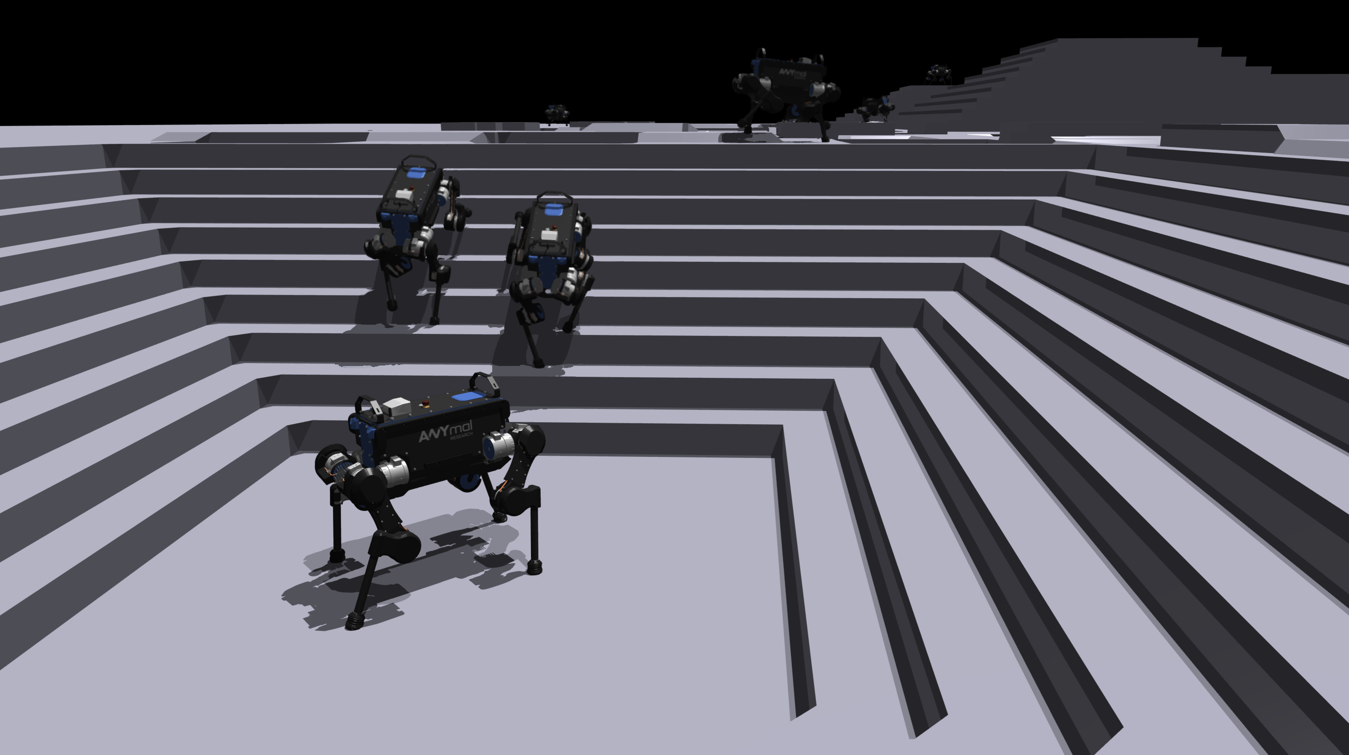
1. Sim-to-real Transfer Became Ready
With Isaac Gym (2021) and domain randomization, training an RL policy in simulation and deploying it to a real robot became feasible. The paper "Learning to Walk in Minutes Using Massively Parallel Deep Reinforcement Learning" (arXiv:2109.11978) by ETHZ showed that just a few minutes of GPU training is needed.
2. End-to-end Learning > Hand-crafted Pipeline
Classical methods require hundreds of parameters for manual tuning: ZMP trajectory parameters, CPG oscillator weights, IK gain tuning, foot placement heuristics... RL learns everything from scratch, needing only a reward function definition.
3. Emergent Behaviors
RL policies develop behaviors that no one designed -- automatically raising feet higher when encountering obstacles, leaning when turning, adjusting gait when terrain changes. These behaviors emerge from optimization, cannot be hand-coded.
4. Generalization
An RL policy trained with domain randomization can work on many different terrains without replanning. ZMP/CPG need redesign for each scenario.
But Classical Knowledge Still Matters
Don't misunderstand -- ZMP, CPG, IK aren't "useless". They're still used:
- Reward shaping: Understanding ZMP helps design better reward functions for RL (penalty when ZMP leaves support polygon)
- CPG + RL: Many new papers combine CPG oscillators as action space structure for RL, like CPG-RL (arXiv:2211.00458) by Bellegarda & Ijspeert
- IK for initialization: IK provides standing pose to initialize RL training
- Safety constraints: ZMP constraints are used as safety monitors in production systems
Next in the Series
This is Part 1 of the Locomotion from Zero to Hero series. You've now grasped the theoretical foundation -- ZMP, CPG, and IK -- and the reasons why RL is replacing them.
In the next post, we'll cover the hottest topic:
- Part 2: RL for Locomotion: PPO, Reward Shaping and Curriculum -- How RL is applied to locomotion from reward design to training pipeline
Related Posts
- RL for Locomotion: PPO, Reward Shaping and Curriculum -- Part 2 of the series
- Quadruped Locomotion: legged_gym to Unitree Go2 -- Part 3: hands-on training and deployment
- Walk These Ways: Adaptive Locomotion One Policy -- Part 4: paper analysis
- RL Basics for Robotics: From Markov to PPO -- RL fundamentals before reading this series
- Simulation for Robotics: MuJoCo vs Isaac Sim vs Gazebo -- Simulator comparison for locomotion training