Why this article matters
In Part 1, we brought up Unitree G1 in MuJoCo through low-level DDS. In Part 2, we converted motion data into MCAP for Foxglove playback. In Part 3, we looked at MPC/WBID signals in PlotJuggler: CoM, contact forces, foot references, and wbid_solve_time.
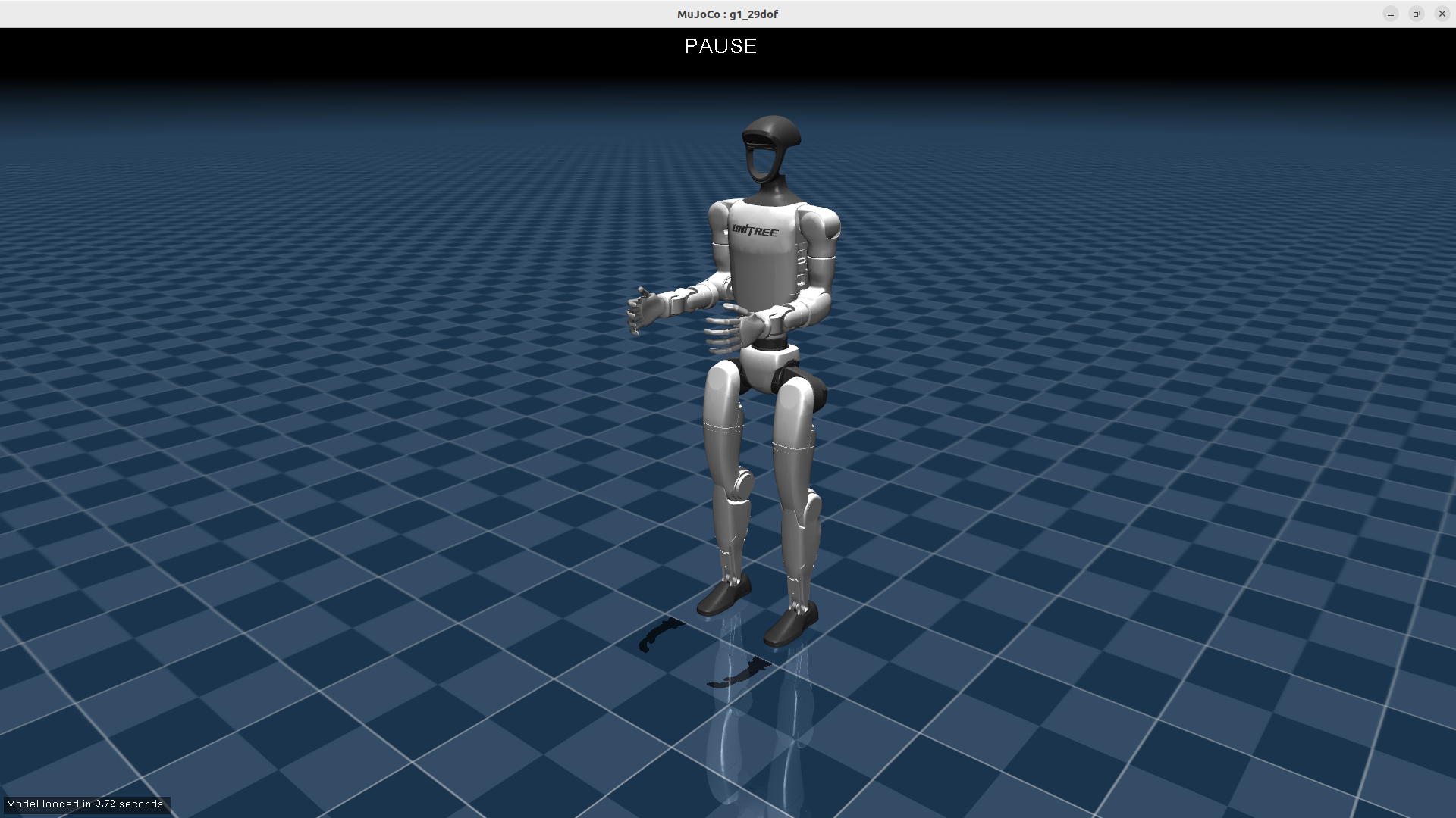
Part 4 moves into the control core. Why can a very short PD controller hold a starting posture, but fail as soon as you ask the robot to walk? Why does a locomotion stack need Whole-Body Inverse Dynamics (WBID) with explicit contact constraints? The main source for this article is ioloizou/g1_locomotion, especially g1_mujoco_sim/src/PD_controller.py and g1_mujoco_sim/src/wbid.py. The repository README describes the framework as a cascaded architecture that combines Single Rigid Body Dynamics (SRBD) and Whole-Body Inverse Dynamics for Unitree G1 in MuJoCo, with the important caveat that the implementation has not yet been tested on the physical robot.
The goal is not to turn you into an optimization expert in one sitting. The practical goal is to read the code without guessing: what each variable means, why Kp/Kd and q_init are only the lowest layer, and why walking requires CoM, Cartesian, DynamicFeasibility, FrictionCone, TorqueLimits, and WrenchLimits.
Series roadmap
The G1 MuJoCo: Control, Foxglove and PlotJuggler series has six parts:
| Part | Article | Main focus |
|---|---|---|
| 1 | Bring Up G1 MuJoCo with Low-Level DDS | Unitree MuJoCo configuration, DDS domain/interface, joystick, and real topics/messages |
| 2 | Convert LAFAN1 G1 Motions to Foxglove MCAP | Convert motion into /tf MCAP for kinematic playback |
| 3 | Debug G1 MPC/WBID with PlotJuggler | Plot SRBD, MPC horizon, contact, foot references, and QP solve time |
| 4 | From Posture PD to Contact-Aware WBID | Compare posture PD with contact-force and constraint-aware WBID |
| 5 | Upper-Body IK for G1 | Control arms and upper body, map joint indices, and check command safety |
| 6 | Sim-to-Real Checklist | Align simulation and hardware: domain, network, gains, timing, and safety |
If you are new to MuJoCo, also read Getting Started with MuJoCo. If you want a broader humanoid software view, Humanoid Robot Software Stack: ROS 2, Isaac and LeRobot is a useful companion article.
q_init: one posture, two different roles
In g1_mujoco_sim/src/config.py, q_init follows the Pinocchio/XBot convention. The vector begins with the 7 floating-base configuration values: position (x, y, z) and quaternion (x, y, z, w). After that come 23 actuated joints: 6 left-leg joints, 6 right-leg joints, 1 waist-yaw joint, 5 left-arm joints, and 5 right-arm joints.
The initial posture is easy to read:
floating base:
  x=0, y=0, z=0.793 - 0.113
  quaternion=(0, 0, 0, 1)

left leg:
  hip_pitch=-0.6, hip_roll=0, hip_yaw=0,
  knee=1.2, ankle_pitch=-0.6, ankle_roll=0

right leg:
  hip_pitch=-0.6, hip_roll=0, hip_yaw=0,
  knee=1.2, ankle_pitch=-0.6, ankle_roll=0

waist:
  waist_yaw=0

arms:
  shoulder/elbow/wrist joints = 0
This is a squat-like standing posture: negative hip pitch, positive knee angle, and negative ankle pitch. It is not a policy, and it is not a gait. It is just a reasonable starting configuration so the MuJoCo model does not begin with locked straight legs.
The important detail is that q_init is used differently by the two controllers:
| Component | How it uses q_init |
Meaning |
|---|---|---|
PD_controller.py |
Uses q_init[7:] as q_desired for all actuated joints |
Pull every joint back to the initial posture |
wbid.py |
Uses the full q_init to initialize the XBot model, FK, initial CoM, and zero velocity |
Build the initial state for inverse dynamics |
PD treats q_init as a fixed target. WBID treats q_init as the model's starting point, then receives references from MPC, the CoM task, base orientation task, contact task, and swing-foot task. This is a major difference. One controller asks, "How far is each joint from the initial posture?" The other asks, "Which whole-body acceleration and contact forces can track the reference without violating dynamics, friction, or actuator limits?"
What the posture PD controller actually does
PD_controller.py is short. It ignores the floating base and reads:
q_current = data.qpos[7:]
q_desired = q_init[7:]
dq_current = data.qvel[6:]
dq_desired = np.zeros(dq_current.shape)
In MuJoCo, the qpos vector of a free-floating humanoid has 7 base position values, while qvel has 6 base velocity values. Actuated joint positions therefore start at qpos[7:], and actuated joint velocities start at qvel[6:]. Beginners often miss this because the base quaternion uses 4 configuration values, while base angular velocity uses only 3 velocity values.
The code then creates two 23-element gain arrays:
Kp[0:6]   = [530, 570, 550, 270, 130, 30]
Kd[0:6]   = [60, 100, 2, 20, 100.5, 5]
Kp[6:12]  = same as the left leg
Kd[6:12]  = same as the left leg
Kp[12]    = 150
Kd[12]    = 10
Kp[13:17] = Kp[18:22] = 20
Kp[17]    = Kp[22] = 11
Kd[13:17] = Kd[18:22] = 5
Kd[17]    = Kd[22] = 0.1
Following the order in q_init, the first 12 values are the two legs, element 12 is waist yaw, and the last 10 values are the two arms. The legs receive large gains because they support the robot's mass. The waist receives medium gains. The arms receive smaller gains because they are not the main ground-force path in a standing posture test.
The final torque command is:
tau = tau_ff + 1.5 * scale * Kp * (q_desired - q_current) \
    + scale / 3 * Kd * (dq_desired - dq_current)
data.ctrl = tau
With scale = 1.5, the effective proportional multiplier is 2.25 * Kp, while the effective damping multiplier is 0.5 * Kd. tau_ff is zero, so this controller does not explicitly compensate gravity, does not use an inertia matrix, does not model Coriolis terms, and does not reason about contact wrenches. It simply pushes every actuated joint toward the desired angle and damps joint velocity.
If the robot is standing with both feet on a flat floor, posture PD may look stable in the viewer. But that stability is narrow. The controller tries to hold joint angles while MuJoCo resolves foot-ground contacts. The controller does not know which foot is in stance, which foot is swinging, how far the CoM has drifted from the support region, whether friction is sufficient, or whether the requested torque exceeds a real actuator limit. When you ask the robot to walk, posture PD pulls the legs back toward the initial posture. It resists the swing motion instead of organizing the contact forces needed for a step.
Why PD is not enough for walking
Walking is not a sequence of independent poses. Walking is contact-rich dynamics. A biped has to do several things at the same time:
- Keep the CoM on a feasible trajectory.
- Control pelvis or torso orientation.
- Keep the stance foot from slipping.
- Move the swing foot toward the landing position.
- Distribute ground reaction forces across heel/toe or contact points.
- Keep friction forces inside the friction cone.
- Keep joint torque within actuator capability.
- Avoid joint and velocity limits.
Posture PD only sees independent joint errors. Even if every joint is close to q_init, the robot can still fall if the CoM is on the wrong side of the stance foot. Conversely, during walking, many joints must deliberately move away from q_init to create a step. If the controller keeps pulling everything back to the old posture, it cancels the motion you need.
A compact mental model is:
Posture PD:
  q_desired - q_current
        |
        v
  23 joint torques

WBID:
  desired CoM, base orientation, stance foot, swing foot, MPC forces
        |
        v
  optimize qddot + contact forces
        |
        v
  inverse-dynamics torques under contact/friction/torque limits
PD is still useful. It is a good baseline for checking the model, joint order, sign convention, and actuator path. But for locomotion, posture PD is missing the entire layer that asks whether the robot is allowed to do the motion in physics.
How WBID builds the optimization problem
In wbid.py, the main class is WholeBodyID. Its constructor takes urdf, dt, q_init, and friction_coef=0.8. It creates an XBot ModelInterface2, reads joint limits, velocity limits, and effort limits from the model, then sets:
self.q = q_init
self.dq = np.zeros(self.model.nv)
The real optimization problem is assembled in WholeBodyID.setupProblem(). The model is first updated at the initial state. Then the code declares the first optimization variable:
variables_vec = dict()
variables_vec["qddot"] = self.model.nv
qddot is the generalized acceleration of the robot. Because the humanoid has a floating base, self.model.nv includes the 6 base velocity-space DOFs plus the actuated joints. This is not just a 23-element joint acceleration vector. WBID solves for full-body acceleration, and inverse dynamics later converts that result into actuator torques.
Next come four 3D contact-force variables:
line_foot_contact_frames = [
    "left_foot_line_contact_lower",
    "left_foot_line_contact_upper",
    "right_foot_line_contact_lower",
    "right_foot_line_contact_upper",
]

for contact_frame in self.contact_frames:
    variables_vec[contact_frame] = 3
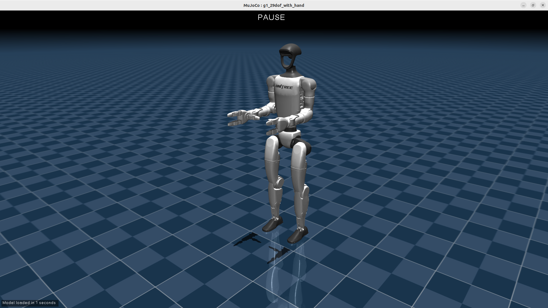
The lower/upper names represent the two line-contact points on each foot. You can think of them as heel/toe-style contact samples along the foot. Two contacts for the left foot and two contacts for the right foot produce 12 force variables in total: Fx, Fy, and Fz for each contact. When ros_run_simulation.py publishes /srbd_current, it uses the same order to attach QP force values to ContactPoint messages.
The tasks inside WBID
After the optimization variables exist, setupProblem() adds tasks. Do not read them as random API calls. Read each task as a control question:
| Task | In the code | Question it answers |
|---|---|---|
| CoM tracking | CoM(self.model, qddot) |
Where should the center of mass be, and with what velocity/acceleration? |
| Base Cartesian orientation | Cartesian("base", ..., "pelvis", qddot) |
Which roll, pitch, and yaw should the pelvis or torso maintain? |
| Contact-foot Cartesian task | Cartesian(left/right_foot_point_contact, ...) |
Should the stance foot remain fixed in the world? |
| Swing-foot Cartesian task | Cartesian(left/right_foot_point_contact, ...) |
Where should the swing foot move? |
| Postural task | Postural(self.model, qddot) |
How should unused or secondary joints stay organized? |
| Angular momentum task | AngularMomentum(...) |
Is body angular momentum being damped instead of drifting? |
| MinimizeVariable tasks | qddot, contact forces, torques |
Can the solution stay smooth and avoid unnecessary force/torque? |
In this stack, CoM receives a large weight (3.*self.com). The postural task is applied only to a subset of indices [18, 19, ..., 28]; it is not pulling the entire robot back to q_init like PD. The base task uses only the orientation part through self.base % [3, 4, 5]. Contact and swing tasks both exist, but ros_run_simulation.py activates or deactivates them according to the gait phase.
This is the subtle difference: WBID still has a posture task, but posture is only a soft preference inside a larger task stack. PD posture turns posture into the entire controller. For humanoid walking, posture should usually mean "keep secondary joints reasonable when there is freedom left," not "override every other objective."
How MPC references enter WBID
When a /mpc_solution message arrives, ros_run_simulation.py unpacks it into:
x_opt[i, 0:3]   = roll, pitch, yaw
x_opt[i, 3:6]   = CoM position
x_opt[i, 6:9]   = angular velocity
x_opt[i, 9:12]  = linear velocity
x_opt[i, 12]    = gravity
u_opt0          = 12 contact-force values, 3 per contact frame
contact_states  = active/inactive flags for the four contacts
During each sim_step, the code updates the model, handles contact phase logic, and then calls:
WBID.stack.update()
WBID.setReference(self.sim_time, self.x_opt[1, :], self.u_opt0, foot_positions_curr)
WBID.solveQP()
tau = WBID.getInverseDynamics()
self.data.ctrl = tau[6:]
setReference() uses x_opt1[0:3] for pelvis orientation, x_opt1[3:6] and x_opt1[9:12] for CoM position and velocity, then computes a CoM acceleration reference from the sum of MPC contact forces divided by robot mass plus gravity. Each wrench_task also receives the 3D force reference for its contact frame.
In other words, MPC does not command "set hip pitch to this angle." MPC provides a centroidal plan: torso orientation, CoM, velocity, and ground reaction forces. WBID turns that plan into full-body acceleration and actuator torque on the full robot model.
Constraints: the part PD does not have
The most important part of wbid.py is not just the task list. It is the constraint list. After the stack is created, the code adds:
DynamicFeasibility
JointLimits
VelocityLimits
TorqueLimits
FrictionCone
WrenchLimits
DynamicFeasibility forces the chosen qddot and contact forces to satisfy floating-base dynamics. For a robot whose base is not directly actuated, this is essential. You cannot arbitrarily ask the pelvis to accelerate sideways if the foot forces and joint torques cannot create that acceleration.
FrictionCone uses friction_coef=0.8. If the tangential contact force is too large relative to the normal force, the foot should slip. PD does not know this. It only produces joint torques. WBID includes contact forces as optimization variables, so it can constrain those forces to remain inside the cone.
TorqueLimits uses effort limits from the URDF. This prevents a solution that looks good numerically but requires impossible actuator torque. WrenchLimits bounds each contact. The default range is [-1000, -1000, 10] to [1000, 1000, 1000], which means the normal force has a positive lower bound while a contact is supporting the robot. When a foot is swinging, ros_run_simulation.py sets the wrench limits for that foot's two contacts to zero so the swing foot cannot still push against the ground.
A quick reading table:
| Constraint | What can go wrong without it? |
|---|---|
DynamicFeasibility |
The QP chooses accelerations that floating-base dynamics cannot produce |
FrictionCone |
The foot asks for excessive lateral force and slips or chatters |
TorqueLimits |
The simulation walks with torque a real actuator could not supply |
WrenchLimits |
The swing foot still "pushes" on the ground, or stance normal force becomes nonsensical |
JointLimits / VelocityLimits |
Joints enter unsafe ranges or produce unrealistic velocities |
MuJoCo's computation and inverse dynamics documentation also emphasizes that contact dynamics cannot be treated as a simple joint-only problem: inverse dynamics in a contact system must account for contact forces and constraints. That is why serious humanoid walking stacks track acceleration, force, friction, and actuator limits, not only joint-angle error.
From the QP solution to data.ctrl
After solveQP(), WBID extracts the solution:
self.ddq = self.variables.getVariable("qddot").getValue(self.x)
self.contact_forces.append(
    self.variables.getVariable(contact_frame).getValue(self.x)
)
Then getInverseDynamics() sets the model acceleration, calls computeInverseDynamics(), and subtracts contact wrench contributions through the contact Jacobians:
tau = self.model.computeInverseDynamics()
for contact_frame:
    Jc = self.model.getJacobian(contact_frame)
    tau = tau - Jc[:3, :].T @ contact_force
return tau
In ros_run_simulation.py, the command sent to MuJoCo is tau[6:], which removes the 6 floating-base DOFs:
self.data.ctrl = tau[6:]
This final line looks similar to PD because both controllers write to data.ctrl. But the path is completely different. PD maps joint error directly to torque. WBID maps MPC/reference signals into a constrained QP, solves for full-body acceleration and contact forces, runs inverse dynamics, and only then produces actuator torque.
Debug checklist when the robot falls
When the robot falls in this stack, do not blindly tune gains. Split the failure by layer:
| Symptom | First suspects |
|---|---|
| The robot cannot stand with PD | Wrong joint order, sign, q_init, timestep, actuator mapping, or gains |
| PD stands, but WBID falls immediately | Wrong MuJoCo/XBot permutation, bad contact frame, infeasible qddot/force QP |
| CoM reference is smooth but current state drifts | Contact force is insufficient, friction cone is tight, torque limits bind, or stance-foot task is weak |
| Swing foot drags | Contact state is wrong, swing task is inactive, or swing-foot wrench limits are not zero |
| Solve time spikes | The stack is over-constrained, constraints conflict, references jump, or the solver receives a hard QP |
This is where Part 3 on PlotJuggler becomes useful again. Plot /mpc_solution, /srbd_current, /feet_ref_pos, and /wbid_statistics/full/statistics[0]/value. If MPC is already bad, fix MPC. If MPC is smooth but WBID cannot track, inspect contact, task weights, and constraints. If WBID solve time grows, do not only increase gains; check whether references are continuous and whether the problem is feasible.
Conclusion
PD_controller.py is a useful baseline because it is short, readable, and verifies the actuator path from Python to MuJoCo. It uses q_init[7:], joint-group Kp/Kd, zero desired velocity, and direct torque assignment to data.ctrl. For posture holding, that is enough to start.
wbid.py solves a different problem: walking with contact. It optimizes qddot and four 3D contact forces, tracks CoM/base/swing/contact references, and constrains the result with dynamic feasibility, friction cones, torque limits, and wrench limits. That is why WBID is much more complex than PD, but it is also why it has a chance of producing physically meaningful walking motion in MuJoCo.
In Part 5, we will move upward into the upper body: once the legs and CoM have control logic, how should arms, waist, and IK connect to the stack without breaking locomotion?