Why Traditional Behavior Cloning Fails
If you've tried teaching a robot to imitate human actions (imitation learning), you know Behavioral Cloning (BC) — simplest approach: collect demonstrations, train supervised learning, predict action from observation. Simple, easy to implement, but fails miserably in many real-world scenarios.
Problem: Multimodal Actions
Imagine: you teach robot to go around obstacle. Demo 1 goes left, Demo 2 goes right — both correct. What does BC with MSE loss learn? Average of two directions — robot goes straight into obstacle.
Demo 1:  ← (go left)    ✓ Correct
Demo 2:  → (go right)   ✓ Correct
BC output: ↑ (average)  ✗ Hits obstacle!
This is multimodal action distribution — same observation has multiple correct actions. BC with Gaussian regression outputs only 1 mode (mean), loses entire diversity in data.
Compounding Errors
Second problem: each prediction is slightly wrong, errors accumulate over time. After 50 steps, robot completely deviates from learned trajectory. This is why BC works in simulation but fails on real robot — real world always has noise and perturbations.

DDPM Basics: Forward Noise and Reverse Denoising
Before understanding Diffusion Policy, need Denoising Diffusion Probabilistic Models (DDPM) — foundation of all diffusion models.
Forward process: Add noise gradually
Given data point x₀ (e.g., action trajectory), forward process adds Gaussian noise over T steps:
x₀ (clean action) → x₁ (little noise) → x₂ → ... → x_T (pure noise)

Each step: x_t = √(1-β_t) · x_{t-1} + √(β_t) · ε
Where: ε ~ N(0, I), β_t is noise schedule
After T steps (usually T=100 or 1000), x_T is almost entirely Gaussian noise — no information left about x₀.
Reverse process: Denoise to generate data
Reverse process learns to go backwards — create clean data from noise:
x_T (noise) → x_{T-1} → ... → x₁ → x₀ (clean action)

Each step: x_{t-1} = μ_θ(x_t, t) + σ_t · z
Where: μ_θ is neural network predicting noise, z ~ N(0, I)
Neural network ε_θ(x_t, t) trained to predict noise ε added at each step t. Simple loss function:
L = E[‖ε - ε_θ(x_t, t)‖²]
Clever idea: model doesn't predict action directly, predicts noise to remove. Through many denoising steps, action "emerges" from noise — like sculptor removing excess stone.
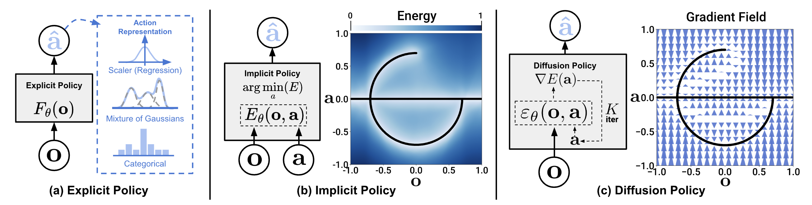
Why diffusion models capture multimodal distributions?
Unlike regression (outputs 1 value), diffusion models learn entire distribution of data. Each sample, process starts from different random noise, leads to different output — naturally captures multiple modes.
Back to obstacle avoidance:
- BC: Always outputs average → hits obstacle
- Diffusion: Sample 1 → go left. Sample 2 → go right. Both valid!
Diffusion Policy: Apply Diffusion to Action Space
Diffusion Policy (Chi et al., RSS 2023) first successful application of diffusion models to robot visuomotor policy learning. Core idea: instead of using diffusion to generate images, use it to generate action trajectories.
Architecture Overview
Observation (image + proprio)
        ↓
   Visual Encoder (ResNet / ViT)
        ↓
   Observation embedding (conditioning)
        ↓
   Conditional Denoising Network
   Input: noisy action chunk A_t^k + timestep k + obs embedding
   Output: predicted noise ε_θ
        ↓
   K denoising steps (DDPM or DDIM)
        ↓
   Clean action chunk A_t^0 = [a_t, a_{t+1}, ..., a_{t+H}]
Important: model predicts entire chunk of actions (e.g., 16 actions in a row) instead of single action. Called action chunking — reduces compounding errors because robot executes whole trajectory smoothly, doesn't need to re-predict every step.
Two Architecture Variants
Paper proposes 2 architectures for denoising network:
1. CNN-based (1D temporal convolution):
# Simplified CNN-based Diffusion Policy
class ConvDiffusionUnet(nn.Module):
    """
    1D U-Net processes action sequence along temporal dimension.
    Similar to image diffusion U-Net but 1D instead of 2D.
    """
    def __init__(self, action_dim=7, obs_dim=512, horizon=16):
        super().__init__()
        # Observation conditioning via FiLM
        self.obs_encoder = nn.Linear(obs_dim, 256)
        # 1D U-Net with residual blocks
        self.down_blocks = nn.ModuleList([
            ResBlock1D(action_dim, 64),
            ResBlock1D(64, 128),
            ResBlock1D(128, 256),
        ])
        self.up_blocks = nn.ModuleList([
            ResBlock1D(256, 128),
            ResBlock1D(128, 64),
            ResBlock1D(64, action_dim),
        ])
        # Timestep embedding
        self.time_embed = SinusoidalPosEmb(256)
- Faster, suited for real-time
- Good for low-dimensional action spaces
2. Transformer-based (Time-series Diffusion Transformer):
# Simplified Transformer-based Diffusion Policy
class DiffusionTransformer(nn.Module):
    """
    Transformer processes action tokens + observation tokens.
    Attention mechanism captures long-range dependencies.
    """
    def __init__(self, action_dim=7, obs_dim=512, horizon=16):
        super().__init__()
        self.action_embed = nn.Linear(action_dim, 256)
        self.obs_embed = nn.Linear(obs_dim, 256)
        self.transformer = nn.TransformerEncoder(
            nn.TransformerEncoderLayer(d_model=256, nhead=8),
            num_layers=6,
        )
        self.action_head = nn.Linear(256, action_dim)
- More flexible, scales better
- Good for high-dimensional tasks and long horizons

Results: Why Diffusion Policy Beats BC by 46.9%
Paper benchmarks on 12 tasks from 4 robot manipulation benchmarks. Impressive results:
| Task Category | BC (LSTM) | BC (Transformer) | IBC | BET | Diffusion Policy |
|---|---|---|---|---|---|
| Push-T | 49.1% | 51.2% | 45.3% | 60.1% | 88.5% |
| Robomimic (Can) | 78.3% | 82.1% | 71.6% | 75.4% | 96.2% |
| Robomimic (Square) | 52.1% | 55.4% | 44.2% | 48.7% | 84.8% |
| Real Robot (Push-T) | 35.0% | 38.2% | 30.1% | 42.3% | 72.1% |
| Average improvement | +46.9% |
Why such huge improvement?
-
Multimodal capture: Diffusion Policy naturally handles multimodal actions — when data has multiple solutions, model samples from distribution instead of averaging.
-
Action chunking + receding horizon: Predict whole chunk of 16 actions, execute 8, re-plan. Reduces compounding errors and creates smooth trajectories.
-
High-dimensional stability: Diffusion more stable than direct regression, especially with large action space (bimanual: 14D+).
-
Training stability: Loss landscape smoother by predicting noise instead of action directly. No need for careful hyperparameter tuning like IBC or EBM methods.
Detailed Training: Action Horizon and Observation Conditioning
Action Horizon and Chunking
Diffusion Policy uses 3 important hyperparameters:
Observation horizon (T_o): Number observation frames = 2
Action horizon (T_a):      Number actions to predict = 16
Action execution (T_e):    Number actions actually execute = 8

Timeline:
  t-1  t  |  t+1  t+2  ...  t+8  |  t+9  ...  t+16
  [obs ]  |  [execute these]      |  [predicted but discarded]
           ↑ re-plan at t+8
Predict 16 but only execute 8, then re-plan with new observation. "Predicted but discarded" part helps model plan ahead — knows trajectory should go somewhere after 8 steps, so first 8 steps will be smoother.
Observation Conditioning
Visual observations encoded by pre-trained ResNet or ViT, then conditioned into denoising network via FiLM conditioning (Feature-wise Linear Modulation):
# FiLM conditioning: obs influences denoising at each layer
gamma = self.gamma_layer(obs_embedding)  # Scale
beta = self.beta_layer(obs_embedding)     # Shift
features = gamma * features + beta        # Modulate
More effective than concatenation because obs embedding influences every layer of network, not just input layer.
Code Example with LeRobot
LeRobot from Hugging Face provides ready Diffusion Policy implementation. Here's how to train and evaluate:
# Install LeRobot
pip install lerobot

# Train Diffusion Policy on PushT task
python lerobot/scripts/train.py \
    --output_dir=outputs/train/diffusion_pusht \
    --policy.type=diffusion \
    --dataset.repo_id=lerobot/pusht \
    --seed=100000 \
    --env.type=pusht \
    --batch_size=64 \
    --steps=200000 \
    --eval_freq=25000 \
    --save_freq=25000

# Evaluate pretrained model
python lerobot/scripts/eval.py \
    --policy.path=lerobot/diffusion_pusht \
    --env.type=pusht \
    --eval.batch_size=10 \
    --eval.n_episodes=10
For custom dataset (collected from real robot):
"""
Train Diffusion Policy on custom robot data with LeRobot
Requires: 1x RTX 3090/4090, dataset in LeRobot format
"""
from lerobot.datasets.lerobot_dataset import LeRobotDataset

# 1. Load dataset (RLDS or LeRobot HDF5 format)
dataset = LeRobotDataset("lerobot/aloha_mobile_cabinet")
print(f"Dataset size: {len(dataset)} frames")
print(f"Action dim: {dataset[0]['action'].shape}")
print(f"Observation keys: {dataset[0]['observation'].keys()}")

# 2. Train with config
# Config file: lerobot/configs/policy/diffusion.yaml
# Key hyperparameters:
#   noise_scheduler: DDPMScheduler (100 diffusion steps)
#   action_horizon: 16 (predict 16 future actions)
#   obs_horizon: 2 (use 2 observation frames)
#   n_action_steps: 8 (execute 8 actions)
#   vision_backbone: "resnet18" (visual encoder)
#   lr: 1e-4

# 3. Deploy on robot
from lerobot.policies.diffusion.modeling_diffusion import DiffusionPolicy
import torch

policy = DiffusionPolicy.from_pretrained("outputs/train/diffusion_pusht/checkpoints/last/pretrained_model")
policy.eval()

# Inference loop
with torch.no_grad():
    obs = get_robot_observation()  # Camera image + proprioception
    action_chunk = policy.select_action(obs)  # [16, action_dim]
    # Execute first 8 actions
    for i in range(8):
        robot.execute(action_chunk[i])
Diffusion Policy vs ACT
ACT (Action Chunking with Transformers) (Zhao et al., RSS 2023) is another prominent approach from similar time period. Comparison:
| Diffusion Policy | ACT | |
|---|---|---|
| Generation method | Iterative denoising (K steps) | Single forward pass (CVAE) |
| Multimodal actions | Native (diffusion distribution) | Via latent variable z |
| Inference speed | Slower (~10-50 denoising steps) | Faster (1 forward pass) |
| Training complexity | Noise scheduling, many hyperparams | Simpler (VAE loss + reconstruction) |
| Precision | Higher via iterative refinement | Good, especially for bimanual |
| Best use case | Complex manipulation, multi-modal | Bimanual, fine-grained tasks |
| Compounding error | Low (action chunking + receding horizon) | Low (action chunking) |
When to use Diffusion Policy?
- Task has multimodal solutions (many ways to solve)
- Need high precision (iterative refinement helps)
- Have enough compute for inference (10+ denoising steps)
When to use ACT?
- Need real-time response (single forward pass)
- Bimanual manipulation (ACT designed for ALOHA)
- GPU inference budget limited
In practice, both are state-of-the-art and often give comparable results. Diffusion Policy has edge on complex multi-modal tasks, ACT has edge on speed and simplicity.
Impact and Follow-up Work
Diffusion Policy opened door to many new research directions:
- 3D Diffusion Policy: Add 3D point cloud observations instead of just 2D images
- Diffusion Policy in VLA models: Octo uses diffusion action head inspired by this paper
- On-device Diffusion Transformer: Optimize diffusion for edge deployment, reduce from 100 steps down to 4-8 with distillation
- Flow matching: pi0 (Physical Intelligence) replaces DDPM with flow matching — faster inference, same quality
Diffusion Policy not just a paper — changed how community thinks about robot learning. From "predict 1 action" to "generate action distribution", from deterministic to stochastic, from single-step to trajectory-level.
Related Posts
- Foundation Models for Robot: RT-2, Octo, OpenVLA in Practice — VLA models overview and fine-tuning
- Sim-to-Real Transfer: Train in Simulation, Run on Real Robot — Transfer policy from sim to real robot
- Robotics Research Trends 2025 — Research landscape overview
- AI and Robotics 2025: Trends and Real-World Applications — AI applications in industrial robots