Psi0 Hands-On (4): Setup & Training Pipeline
After understanding the data recipe in the previous post, it is time to get our hands dirty: setting up the environment, downloading model checkpoints, and running Psi0's 3-stage training pipeline. This post walks you through the entire process — from git clone to having a fine-tuned model ready for deployment.
Hardware Requirements
Before getting started, determine which category you fall into:
| Purpose | Minimum GPU | VRAM | Notes |
|---|---|---|---|
| Inference only | 1x RTX 4090 | 24 GB | Run a pre-trained model |
| Fine-tune (Stage 3) | 2x A100 40GB | 80 GB | Most practical for individuals |
| Post-train (Stage 2) | 32x A100 80GB | 2.5 TB | Requires a cluster |
| Pre-train (Stage 1) | 64x A100 80GB | 5 TB | Requires a large cluster |
Reality check: Most people will only run Stage 3 (Fine-tune) using pre-trained checkpoints provided by the authors. This is also the most practical part — you only need 2-8 GPUs to fine-tune for your own new task.
If you do not have access to powerful GPUs, popular cloud providers include:
- Lambda Labs: ~$1.1/hour for A100 80GB
- RunPod: ~$1.6/hour for A100 80GB
- Vast.ai: ~$0.8/hour for A100 40GB (spot pricing)
Environment Setup
Step 1: Clone the Repository
git clone https://github.com/physical-superintelligence-lab/Psi0.git
cd Psi0
Step 2: Install the uv Package Manager
Psi0 uses uv instead of traditional pip/conda. uv is 10-100x faster than pip and handles dependencies more reliably:
# Install uv
curl -LsSf https://astral.sh/uv/install.sh | sh

# Verify
uv --version
Step 3: Create a Virtual Environment with Python 3.10
# Create venv with Python 3.10 (required)
uv venv --python 3.10
source .venv/bin/activate

# Verify Python version
python --version  # Must be 3.10.x
Why Python 3.10? Flash Attention 2.7.4 and certain CUDA extensions only have stable support on Python 3.10. Python 3.11+ can cause compilation errors.
Step 4: Install Dependencies
# Install core dependencies
uv pip install -e .

# Install Flash Attention (required, needs CUDA toolkit)
uv pip install flash-attn==2.7.4 --no-build-isolation

# Verify Flash Attention
python -c "import flash_attn; print(flash_attn.__version__)"
# Output: 2.7.4
Important note: Flash Attention requires the CUDA toolkit to be installed on your system (not just PyTorch's CUDA runtime). If you encounter compilation errors:
# Check CUDA toolkit
nvcc --version  # Need 11.8 or 12.x

# If not installed:
# Ubuntu:
sudo apt install nvidia-cuda-toolkit

Step 5: Configure Environment Variables
Create a .env file in the project root directory:
# .env file
export HF_TOKEN=hf_xxxxxxxxxxxxxxxxxxxxxxxxxxxxxxxx
export WANDB_API_KEY=xxxxxxxxxxxxxxxxxxxxxxxxxxxxxxxx
export PSI_HOME=/path/to/Psi0
HF_TOKEN: Obtain from huggingface.co/settings/tokens. You need read access to download models and data.
WANDB_API_KEY: Obtain from wandb.ai/settings. Used for monitoring training — critically important since training runs can last for days.
PSI_HOME: Absolute path to the Psi0 directory. Scripts use this variable to locate configs, checkpoints, and data.
# Load env vars
source .env

# Verify
echo $HF_TOKEN   # Should display your token
echo $PSI_HOME    # Should display the path
Step 6: Log in to HuggingFace and W&B
# Login to HuggingFace
huggingface-cli login --token $HF_TOKEN

# Login to Weights & Biases
wandb login $WANDB_API_KEY
Downloading Model Checkpoints and Data
Download Pre-trained Checkpoints
# Download System-2 (Qwen3-VL-2B, fine-tuned)
python scripts/data/download_checkpoints.py \
  --repo_id physical-superintelligence/psi0-system2 \
  --local_dir checkpoints/system2

# Download System-1 (MM-DiT action expert)
python scripts/data/download_checkpoints.py \
  --repo_id physical-superintelligence/psi0-system1 \
  --local_dir checkpoints/system1

# Download System-0 (RL locomotion controller)
python scripts/data/download_checkpoints.py \
  --repo_id physical-superintelligence/psi0-system0 \
  --local_dir checkpoints/system0
Download Training Data
# Simulation data (smaller, use to test the pipeline)
python scripts/data/download_datasets.py \
  --repo_id physical-superintelligence/psi0-sim-data \
  --local_dir data/sim

# Real-world data (larger, needed for real fine-tuning)
python scripts/data/download_datasets.py \
  --repo_id physical-superintelligence/psi0-real-data \
  --local_dir data/real
Note: Data downloads can take several hours depending on network speed. EgoDex (829 hours of video) is very large — only download it if you truly need to pre-train from scratch.
Stage 1: Pre-training (64x A100)
Purpose
Stage 1 teaches System-2 (Qwen3-VL-2B) to understand manipulation primitives from egocentric video (EgoDex) and robot data (HE). The model learns autoregressively — predicting the next FAST token based on images + previous tokens.
Hyperparameters
| Parameter | Value | Explanation |
|---|---|---|
| GPUs | 64x A100 80GB | Distributed training with FSDP |
| Batch size | 1024 | Global batch size (16 per GPU) |
| Learning rate | 1e-4 | AdamW optimizer |
| Steps | 200,000 | ~3-4 days of training |
| Warmup | 2000 steps | Linear warmup |
| Scheduler | Cosine decay | Decay to 1e-6 |
Running Pre-training
# Pre-train (REQUIRES 64x A100)
torchrun --nproc_per_node=8 --nnodes=8 \
  scripts/train/psi0/pretrain-psi0.sh

# Or use SLURM
sbatch scripts/train/psi0/pretrain-psi0.slurm
Reality check: You almost certainly do not need to run Stage 1. The authors have provided pre-trained checkpoints. Use the available checkpoint and jump straight to Stage 2 or Stage 3.
What If You Don't Have 64 GPUs?
Use the pre-trained checkpoint:
# Download pre-trained Stage 1 checkpoint
python scripts/data/download_checkpoints.py \
  --repo_id physical-superintelligence/psi0-pretrained \
  --local_dir checkpoints/pretrained
This checkpoint contains Qwen3-VL-2B already trained on EgoDex + HE, ready for Stage 2 or Stage 3.
Stage 2: Post-training — Flow Matching (32x A100)
Purpose
Stage 2 trains System-1 — the MM-DiT (Multi-Modal Diffusion Transformer) action expert with 500M parameters. This is the model responsible for generating precise joint-space actions based on features from System-2.
The critical point: the VLM (System-2) is frozen at this stage. Only the MM-DiT is trained. The VLM serves as the "eyes and brain" — observing the scene and producing a representation. The MM-DiT learns to translate that representation into concrete actions.
What Is Flow Matching?
Flow Matching is a generative modeling method similar to Diffusion but more efficient. Instead of adding noise and then denoising (like DDPM), Flow Matching learns a vector field that transforms from a noise distribution to an action distribution along a straight path.
Pseudocode for the Flow Matching training loop:
# Pseudocode: Flow Matching Training Loop
for batch in dataloader:
    images = batch["observation.images"]      # [B, C, H, W]
    states = batch["observation.state"]        # [B, 28]
    target_actions = batch["action"]           # [B, T, 36] (T timesteps)

    # 1. VLM encode (frozen, no gradient)
    with torch.no_grad():
        vlm_features = system2.encode(images)  # [B, D]

    # 2. Sample random timestep t ~ Uniform(0, 1)
    t = torch.rand(B, device=device)           # [B]

    # 3. Sample noise
    noise = torch.randn_like(target_actions)   # [B, T, 36]

    # 4. Interpolate: x_t = (1-t) * noise + t * target
    x_t = (1 - t.unsqueeze(-1).unsqueeze(-1)) * noise + \
          t.unsqueeze(-1).unsqueeze(-1) * target_actions

    # 5. Predict velocity field v(x_t, t, condition)
    v_pred = mmdit(x_t, t, vlm_features, states)  # [B, T, 36]

    # 6. Target velocity = target - noise (straight line)
    v_target = target_actions - noise

    # 7. MSE loss
    loss = F.mse_loss(v_pred, v_target)

    loss.backward()
    optimizer.step()
Stage 2 Hyperparameters
| Parameter | Value |
|---|---|
| GPUs | 32x A100 80GB |
| Batch size | 2048 (global) |
| Learning rate | 1e-4 |
| Steps | 30,000 |
| Warmup | 1000 steps |
Running Post-training
# Post-train MM-DiT (REQUIRES 32x A100)
torchrun --nproc_per_node=8 --nnodes=4 \
  scripts/train/psi0/posttrain-psi0.sh
As with Stage 1, you can use the pre-existing Stage 2 checkpoint instead of training from scratch.

Stage 3: Fine-tuning — The Most Practical Part!
This is the stage that most people will actually run. Stage 3 fine-tunes the entire pipeline (System-2 + System-1) on 80 demonstrations of a specific task.
Stage 3 Hyperparameters
| Parameter | Value | Adjustable? |
|---|---|---|
| GPUs | 2-8x A100/H100 | Fewer GPUs -> increase gradient accumulation |
| Batch size | 128 (global) | Split evenly across GPUs |
| Learning rate | 1e-4 | Use cosine schedule |
| Steps | 40,000 | ~6-8 hours on 4x A100 |
| Warmup | 500 steps | Linear warmup |
| LR scheduler | Cosine decay | Decay to 0 |
| Weight decay | 0.01 | AdamW |
Fine-tuning in Simulation
# Fine-tune on simulation data
bash scripts/train/psi0/finetune-simple-psi0.sh \
  --data_dir data/sim/pick_place \
  --checkpoint_dir checkpoints/pretrained \
  --output_dir outputs/sim_pick_place \
  --num_gpus 4 \
  --batch_size 128 \
  --lr 1e-4 \
  --max_steps 40000 \
  --warmup_steps 500
Fine-tuning on Real-World Data
# Fine-tune on real robot data
bash scripts/train/psi0/finetune-real-psi0.sh \
  --data_dir data/real/fold_clothes \
  --checkpoint_dir checkpoints/pretrained \
  --output_dir outputs/real_fold_clothes \
  --num_gpus 2 \
  --batch_size 128 \
  --lr 1e-4 \
  --max_steps 40000
Adjusting Batch Size Based on GPU Count
The batch size of 128 is the global batch size. If you have fewer GPUs, use gradient accumulation:
# 8 GPUs: batch_per_gpu = 128 / 8 = 16
--num_gpus 8 --batch_size_per_gpu 16 --gradient_accumulation 1

# 4 GPUs: batch_per_gpu = 128 / 4 = 32 (if VRAM allows)
--num_gpus 4 --batch_size_per_gpu 32 --gradient_accumulation 1

# 4 GPUs, limited VRAM: use gradient accumulation
--num_gpus 4 --batch_size_per_gpu 16 --gradient_accumulation 2

# 2 GPUs: more gradient accumulation
--num_gpus 2 --batch_size_per_gpu 16 --gradient_accumulation 4

# 1 GPU (slow but works):
--num_gpus 1 --batch_size_per_gpu 16 --gradient_accumulation 8
Rule of thumb: num_gpus x batch_size_per_gpu x gradient_accumulation = 128 (global batch size). Gradient accumulation slows down training but produces equivalent results.
Monitoring Training with Weights & Biases
W&B is an indispensable tool when training runs last for hours or days. Psi0 comes with built-in W&B logging.
Loss Curves to Monitor
During training, you will see the following metrics on your W&B dashboard:
1. Total Loss (train/loss)
- Drops rapidly in the first 5,000 steps
- Decreases slowly and stabilizes after 20,000 steps
- If loss spikes suddenly -> learning rate is too high or there is a data issue
2. Action Loss (train/action_loss)
- MSE loss between predicted and target actions
- Should drop below 0.01 after 30,000 steps
- If it plateaus early (>0.05 after 10,000 steps) -> data quality issue
3. Learning Rate (train/lr)
- Cosine curve: linear increase during warmup, then gradual cosine decrease
- Verify the LR schedule is correct — an incorrect LR schedule is a common cause of training failure
Signs of Healthy Training
Step 1000:  loss=0.85, action_loss=0.12  <- Rapid decrease, good
Step 5000:  loss=0.32, action_loss=0.04  <- Continuing to decrease
Step 10000: loss=0.18, action_loss=0.02  <- Starting to converge
Step 20000: loss=0.11, action_loss=0.008 <- Near convergence
Step 40000: loss=0.08, action_loss=0.005 <- Converged
Signs of Training Problems
Step 1000:  loss=0.85  <- OK
Step 2000:  loss=NaN   <- LR too high! Reduce LR by 10x
Step 1000:  loss=0.85  <- OK
Step 5000:  loss=0.82  <- Very slow decrease
Step 10000: loss=0.80  <- Plateaued too early -> check data
Checkpoint Management
Saving Checkpoints
Training automatically saves checkpoints every N steps (configurable). Each checkpoint is roughly 4-6 GB:
# Output directory structure
outputs/sim_pick_place/
├── checkpoint-5000/
│   ├── model.safetensors
│   ├── optimizer.pt
│   └── training_state.json
├── checkpoint-10000/
├── checkpoint-20000/
├── checkpoint-30000/
├── checkpoint-40000/   <- Final checkpoint
└── logs/
    └── events.out.tfevents.*
Resuming Training
If training is interrupted (OOM, server restart, spot instance preempted):
# Resume from the latest checkpoint
bash scripts/train/psi0/finetune-simple-psi0.sh \
  --data_dir data/sim/pick_place \
  --checkpoint_dir outputs/sim_pick_place/checkpoint-20000 \
  --output_dir outputs/sim_pick_place \
  --resume_from_checkpoint true \
  --max_steps 40000
Selecting the Best Checkpoint
The final checkpoint is not always the best. Sometimes the model overfits toward the end of training. Here is how to choose:
- Check validation loss on W&B — select the checkpoint with the lowest validation loss
- Evaluate on held-out episodes — run inference on 5-10 episodes not used for training
- If no validation set is available — the checkpoint at 80% of training (step 32,000) is typically a safe choice
# Evaluate a checkpoint
python scripts/eval/evaluate_checkpoint.py \
  --checkpoint_dir outputs/sim_pick_place/checkpoint-30000 \
  --eval_data data/sim/pick_place_eval \
  --num_episodes 10
Troubleshooting Common Issues
1. Out of Memory (OOM)
CUDA out of memory. Tried to allocate 2.00 GiB
Solutions (in order of priority):
- Reduce
batch_size_per_gpu(16 -> 8 -> 4) - Increase
gradient_accumulationaccordingly - Enable
gradient_checkpointing(saves VRAM, ~20% slower) - Reduce
max_seq_lengthif the config allows
# Example: OOM with batch 16 on A100 40GB
--batch_size_per_gpu 8 --gradient_accumulation 2 --gradient_checkpointing true
2. NaN Loss
Step 3456: loss=NaN
Common causes: Learning rate too high, data contains outlier values, or mixed precision issues.
Solutions:
- Reduce learning rate by 10x (1e-4 -> 1e-5)
- Validate data:
python scripts/data/validate_dataset.py --data_dir data/... - Disable mixed precision (bf16 -> fp32) — 2x slower but stable
- Increase warmup steps (500 -> 2000)
3. Training Too Slow
| Bottleneck | Symptoms | Solution |
|---|---|---|
| Data loading | GPU utilization < 50% | Increase num_workers, use SSD |
| GPU compute | GPU util 100%, high step time | Enable Flash Attention, reduce seq length |
| Communication | Multi-GPU step time >> single GPU | Check NCCL bandwidth, use NVLink |
# Monitor GPU utilization
watch -n 1 nvidia-smi

# If GPU util is low -> increase data loading workers
--num_workers 8  # Instead of default 4
4. Checkpoints Too Large
Each checkpoint is 4-6 GB, saving every 5,000 steps = 40-48 GB for full training. Solutions:
# Keep only the N most recent checkpoints
--save_total_limit 3

# Or save less frequently
--save_steps 10000  # Instead of 5000
Real-Time Chunking for Deployment
After training is complete, the model needs to run in real-time on the robot. Psi0 uses Real-Time Chunking to achieve 160ms latency:
# Pseudocode: Real-Time Chunking Inference
action_buffer = []
chunk_size = 16  # Predict 16 timesteps at once

while robot_running:
    if len(action_buffer) == 0:
        # Buffer empty -> predict new chunk
        images = camera.capture()
        state = robot.get_state()

        # VLM encode + MM-DiT generate (~160ms)
        action_chunk = model.predict(images, state)  # [16, 36]
        action_buffer = list(action_chunk)

    # Pop the first action from the buffer
    action = action_buffer.pop(0)
    robot.execute(action)  # 50Hz control loop

    # Overlap: start predicting the next chunk
    # while still executing actions from the current buffer
Key insight: The model predicts 16 actions at once (an action chunk). The robot executes each action at 50Hz (20ms/action). While executing 16 actions (320ms), the model has enough time to predict the next chunk (160ms). There is no delay between chunks.
This approach differs from traditional Diffusion Policy which requires 100+ denoising steps. Psi0's Flow Matching only needs 4-8 steps per chunk, making it significantly faster.

Summary: From Code to Robot
Here is the complete workflow in summary:
1. Clone repo + install uv + Python 3.10 + Flash Attention
2. Configure .env (HF_TOKEN, WANDB_API_KEY, PSI_HOME)
3. Download pre-trained checkpoints (skip Stage 1 & 2)
4. Collect 80 demos for your task
5. Convert to LeRobot format (raw_to_lerobot.py)
6. Fine-tune Stage 3 (2-8 GPUs, ~6-8 hours)
7. Monitor on W&B, select the best checkpoint
8. Deploy with Real-Time Chunking (160ms latency)
With this workflow, you can go from "nothing" to "robot performing a new task" in a few days — most of the time is spent collecting 80 demos and waiting for training to finish. This is a significant improvement over previous methods that required thousands of demos and weeks of training.
Psi0 is not just a great paper — it is an open framework that anyone with GPUs and a robot can use. With the LeRobot format standardizing data, the community can share datasets and checkpoints, accelerating humanoid robot research and applications worldwide.
Related Posts
- Psi0 Hands-On (3): Data Recipe & Pipeline — Understanding the 3-tier data recipe and why 860h of data beats 10,000h
- VLA + LeRobot (1): Framework Overview — The LeRobot format foundation that Psi0 uses for its entire data pipeline
- Diffusion Policy: Generating Actions for Robots — Comparing Flow Matching with Diffusion — two generative modeling paradigms for robots