A robot reaching for a cup does not need every part of the table to receive equal computational attention throughout the movement. Finding the cup may require a broad view. Closing the gripper may depend more heavily on a small interaction region. Yet a Vision-Language-Action model can repeatedly send a long visual sequence through its language backbone whenever it predicts another action.
FastVLA, by Jiuyi Xu and colleagues, tackles this cost with task-conditioned, temporally adaptive visual token pruning. It retains an existing policy and adds an inference-time decision about which visual tokens to keep and how many are necessary for the current prediction. This tutorial walks through the algorithm and a practical OpenVLA-OFT evaluation on LIBERO, without requiring you to train a VLA from scratch.
Start with the original FastVLA paper and jiuyixu25/FastVLA repository. Check the authors and repository when searching: a different project named Fast-VLA uses task memory. This article concerns adaptive visual token compression. Numerical results below are the authors' published measurements, not measurements reproduced on our own hardware.
1. Three concepts to understand first
A visual token is a vector representing information extracted from an image. A vision encoder produces visual features, and a projector maps them into a representation accepted by the language backbone. Multiple camera views generally increase the sequence length and the amount of downstream computation.
Closed-loop control means observing the scene, predicting actions, executing them, and observing again. Policy latency affects how frequently a robot can react to changes. A policy with excellent offline accuracy may still struggle when feedback arrives too slowly after an object slips or becomes occluded.
An action chunk contains several actions predicted in one model call. The OpenVLA-OFT configuration evaluated here predicts eight actions per call. Actions executed per second and fresh model predictions per second therefore describe different things. For a broader introduction to the image-to-action pipeline, see our OpenVLA explanation.
For the hands-on section, use a Linux machine with an NVIDIA GPU and a CUDA setup compatible with PyTorch. The README describes LIBERO evaluation using one GPU with approximately 16 GB of memory; published performance comes from an RTX 4090. Treat this as environment guidance, rather than a guarantee that every 16 GB card will support every configuration or deliver the reported latency.
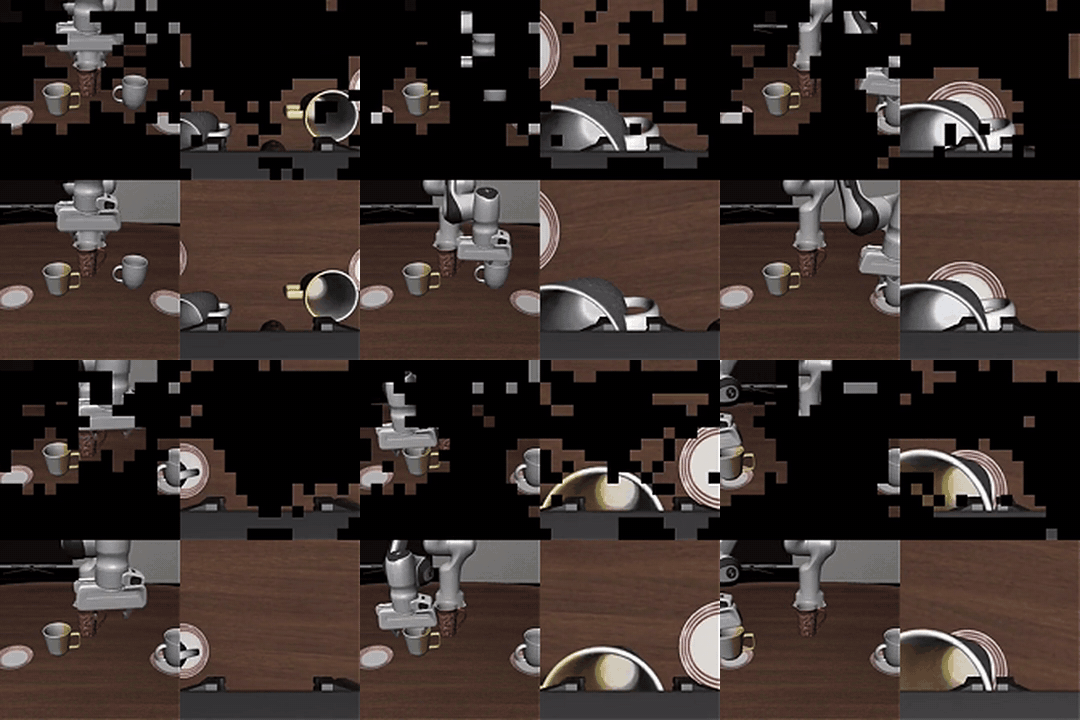
The repository animation shows the distinction between the complete observation and the tokens forwarded through the LLM. Black regions indicate discarded tokens; the camera still captures the original image.
2. Where FastVLA fits in the architecture
The conceptual processing path is:
Camera images -> vision encoder -> projector -> visual tokens
                                                    |
Instruction -> task embeddings --------------------+-> FastVLA
                                                         |
                                       BOS + retained visual tokens
                                             + task tokens
                                                         |
                                                   LLM backbone
                                                         |
                                                     action head
                                                         |
                                              action chunk -> robot
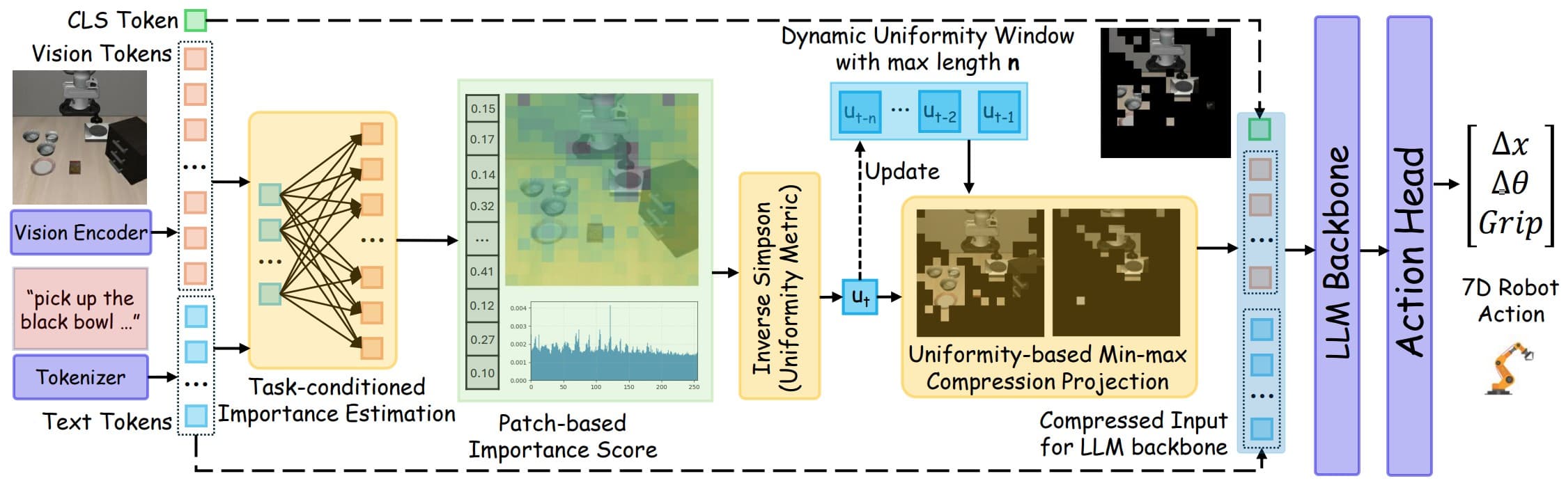
This diagram abstracts integration-specific inputs such as proprioception. The core module expects a sequence arranged as [BOS | N visual tokens | task tokens]. It preserves the beginning-of-sequence token and task span while shortening the visual span. Selected visual tokens retain their original order and position IDs. Sorting the resulting sequence by importance would change the positional structure expected by the policy.
Placement also explains the limits of acceleration. The vision encoder must produce features before FastVLA can score them. Pruning reduces language-backbone work; it does not eliminate image acquisition, preprocessing, visual encoding, or action-head computation. Read the standalone core implementation when integrating the method into another policy.
3. How the adaptive budget works
Score tokens using the instruction
FastVLA applies RMS normalization to task and visual embeddings, computes their scaled dot products, normalizes over visual tokens with softmax, and averages across task tokens:
A = softmax(RMSNorm(T) @ RMSNorm(V).T / sqrt(d), visual_axis)
s[i] = mean(A[:, i], task_axis)
Here, T represents task embeddings, V represents image embeddings, and d is the hidden dimension. A high score means a visual token receives relatively strong attention from the task representation. This score is computed from embeddings at the LLM input; it does not require running the full decoder to extract attention from a deep layer.
Intuitively, placing a cup on a plate should make the cup, plate, and interaction area more useful than unrelated table texture. Attention remains an approximation of control relevance, however. A low score does not prove that removing a token is harmless. Rollout success must still be checked after changing the token budget.
Measure concentration with inverse Simpson uniformity
Suppose a few tokens receive almost all the importance. Keeping a large sequence may be wasteful. If importance is spread more evenly, a small retained set could lose necessary context. FastVLA summarizes concentration over the highest-scoring tokens:
K = ceil((1 - (rho + tau)) * N)
q[j] = top_score[j] / sum(top_scores)
K_eff = 1 / sum(q[j] ** 2)
U = K_eff / K
For a simple mathematical example, four equal normalized weights of 0.25 give an effective count of four and U=1. If one weight takes nearly all the mass, the effective count approaches one. These are illustrative calculations, not measured rollout values.
The reference K in this calculation is not the final retained-token count. It measures concentration using the smallest budget allowed by the configured rate band. The implementation clamps it to at least one. The actual retained budget is chosen afterward and can change at every prediction.
Turn concentration into a pruning rate
rho specifies the target fraction removed, tau defines the allowed variation, and window specifies how many previous uniformity values are stored. FastVLA compares the current value with the minimum and maximum of the previous values:
alpha = clip((U - U_min) / (U_max - U_min), 0, 1)
rate = rho + tau - 2 * tau * alpha
kept = max(1, round((1 - rate) * N))
Relatively concentrated evidence produces more aggressive pruning. Relatively uniform evidence produces a more conservative decision. The first two predictions use rho - tau because the calibration history is not yet populated. When the historical range is effectively zero, the implementation uses rho rather than dividing by zero.
For an illustrative sequence of 512 visual tokens, rho=0.8 and tau=0.1 allow removal rates between 70% and 90%, leaving approximately 154 to 51 tokens after rounding. Crucially, rho=0.8 means removing 80%, not retaining 80%. The realized average removal rate need not equal the nominal target exactly.
FastVLA does not reuse cached visual features between control steps. Its temporal state is a short calibration history. Reset that history at every new episode. The current core processes one episode stream with batch size one, so independent simultaneous rollouts need independent state handling.
4. Install the evaluation environment
The following commands are instructions for your experiment machine, based on the repository installation guide. First inspect the GPU and create a separate environment:
nvidia-smi
conda create -n fastvla python=3.10 -y
conda activate fastvla

# Select the PyTorch CUDA wheel appropriate for your driver.
pip install torch==2.2.0 torchvision==0.17.0 torchaudio==2.2.0

git clone https://github.com/jiuyixu25/FastVLA.git
cd FastVLA
pip install -e .
An editable installation makes the local checkout importable as a Python package. Keep the environment active for subsequent commands. Install LIBERO and the simulator packages next:
git clone https://github.com/Lifelong-Robot-Learning/LIBERO.git
pip install -e LIBERO
pip install -r experiments/robot/libero/libero_requirements.txt
pip install bddl==1.0.1 mujoco==2.3.2 gym==0.25.2 robosuite==1.4.1

# Make local packages discoverable from the FastVLA root directory.
export PYTHONPATH="$PWD:$PWD/LIBERO${PYTHONPATH:+:$PYTHONPATH}"

python -c "import torch, libero; from fastvla import FastVLA; print('CUDA:', torch.cuda.is_available())"
Pinning simulator dependencies is part of reproducibility. Newer releases can change task outcomes even for an uncompressed baseline. If TensorFlow reports a NumPy compatibility problem, the README recommends pip install numpy==1.26.4 opencv-python==4.10.0.84. Apply that workaround when needed, then inspect remaining dependency issues with pip check.
Also inspect pyproject.toml. The OFT integration uses the transformers-openvla-oft fork for bidirectional attention. Replacing it with the newest standard Transformers release can break assumptions in this stack. If your runtime requires FlashAttention, follow the upstream OFT environment instructions after the editable installation; the package notes reference flash-attn==2.5.5. Building CUDA extensions requires a compatible toolkit, not simply a driver visible in nvidia-smi.
On first use, LIBERO may ask where configuration and assets should live. Complete its setup and confirm those paths point to the actual LIBERO checkout. Evaluating an existing checkpoint does not require downloading all demonstration datasets for training, but the simulator still needs its task assets and initial states.
5. Training: what you can skip
There is no FastVLA training stage in this workflow. You do not train a compressor with backpropagation before enabling pruning. Instead, you load a policy checkpoint already adapted to a LIBERO suite, preserve its weights, and apply token selection during inference.
Training-free acceleration does not imply an untrained robot policy. The checkpoint moojink/openvla-7b-oft-finetuned-libero-spatial already contains learned behavior for its benchmark setting. FastVLA reduces the computational cost of using that behavior; an instruction alone does not create a new manipulation skill.
For a different robot, first collect demonstrations and adapt the underlying policy using the appropriate OpenVLA-OFT workflow. Confirm that the baseline works with your cameras, proprioception, and action normalization. Only then enable FastVLA and measure the efficiency–success trade-off. The repository describes its Franka Research 3 experiment as using an OpenVLA-OFT policy fine-tuned with LoRA on teleoperated demonstrations. That training belongs to the base policy, while token compression remains training-free.
Our VLA-Adapter tutorial explains a different part of the workflow: adapting policy capabilities. Keep adaptation and inference acceleration separate during experiments. Changing the checkpoint and pruning strategy simultaneously makes a success-rate difference difficult to interpret.
6. Run inference: establish a baseline first
From the FastVLA repository root, begin with a small baseline run to check checkpoint loading, environment rendering, and rollout completion:
python experiments/robot/libero/run_libero_eval.py \
  --pretrained_checkpoint moojink/openvla-7b-oft-finetuned-libero-spatial \
  --task_suite_name libero_spatial \
  --fastvla_enable False \
  --num_trials_per_task 2 \
  --seed 7 \
  --run_id_note baseline-smoke
Two trials per task are a smoke test, not a reproduction of the paper. Once the baseline runs successfully, enable pruning while keeping the checkpoint, suite, and seed unchanged:
python experiments/robot/libero/run_libero_eval.py \
  --pretrained_checkpoint moojink/openvla-7b-oft-finetuned-libero-spatial \
  --task_suite_name libero_spatial \
  --fastvla_rho 0.8 \
  --fastvla_tau 0.1 \
  --fastvla_window 10 \
  --num_trials_per_task 2 \
  --seed 7 \
  --run_id_note fastvla-smoke
The evaluation configuration defaults to two input images, proprioception, and a continuous action head using L1 regression. Do not reduce the camera count merely to save memory if the checkpoint expects another configuration. Preserve preprocessing and action un-normalization while establishing your initial comparison.
After the smoke test, evaluate all four suites using the supplied runner:
# Defaults to 50 trials per task, with 10 tasks in each suite.
bash scripts/eval_libero_fastvla.sh --seed 7

# Obtain the corresponding uncompressed baseline.
bash scripts/eval_libero_fastvla.sh --seed 7 --fastvla_enable False
| Suite | CLI name | OFT rho | tau | window |
|---|---|---|---|---|
| Spatial | libero_spatial |
0.80 | 0.10 | 10 |
| Object | libero_object |
0.70 | 0.10 | 10 |
| Goal | libero_goal |
0.75 | 0.10 | 10 |
| Long | libero_10 |
0.60 | 0.10 | 10 |
These rates are specific to OpenVLA-OFT. For the original OpenVLA backbone, the README lists 0.35, 0.50, 0.40, and 0.30 respectively, and provides a separate integration. Do not combine an original OpenVLA checkpoint with the OFT evaluation stack merely because both names contain OpenVLA. Their model interfaces and dependency expectations differ.
7. Interpret the results correctly
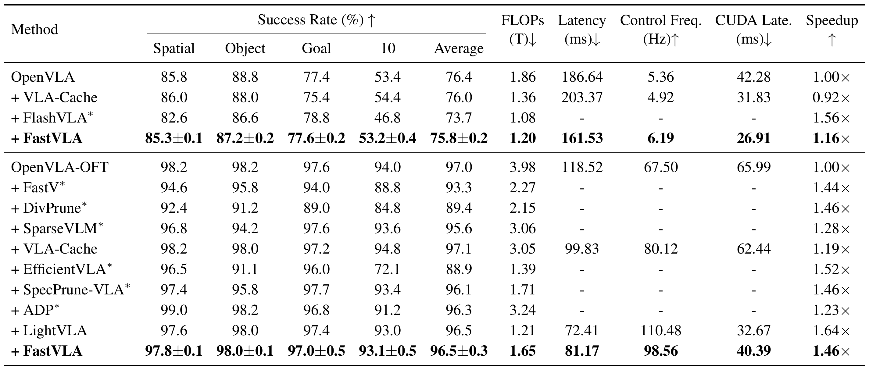
The authors report these aggregate measurements on an RTX 4090:
| Policy | Average success | LLM FLOPs | Action latency | Speedup |
|---|---|---|---|---|
| OpenVLA | 76.4% | 1.86 T | 186.64 ms | 1.00× |
| OpenVLA + FastVLA | 75.8 ± 0.2% | 1.20 T | 161.53 ms | 1.16× |
| OpenVLA-OFT | 97.0% | 3.98 T | 118.52 ms | 1.00× |
| OpenVLA-OFT + FastVLA | 96.5 ± 0.3% | 1.65 T | 81.17 ms | 1.46× |
FastVLA success is reported as mean ± standard error over three seeds. OFT loses 0.5 percentage points of average success, so “comparable success” should not be read as identical outcomes. Its LLM FLOPs fall by approximately 58.5%, while action latency falls by approximately 31.5%. Other pipeline components explain why these percentages differ. Source: published repository results.
You can verify the headline speedup directly: 118.52 / 81.17 ≈ 1.46. With eight actions per chunk, 8 / 0.08117 ≈ 98.56 actions per second. However, the model produces only about 1 / 0.08117 ≈ 12.32 fresh chunks per second. This is not a camera-feedback loop running at 98.56 new observations per second. Execution scheduling and robot dynamics further affect the deployed system.
The evaluator writes text logs and JSON summaries under experiments/logs/. Record success, total action-prediction latency, LLM CUDA latency, FLOPs, and actual retained-token count together. Comparing the backbone-only CUDA time of one method with the full prediction time of another produces a misleading speedup. Record each seed and episode count so that a quick smoke test cannot be mistaken for a benchmark reproduction.
A useful follow-up is a budget-matched comparison between adaptive and fixed pruning. Give the fixed strategy the same average number of tokens consumed by the adaptive run. This tests whether an improvement comes from allocating tokens at better moments, rather than simply retaining more tokens overall. Reporting only nominal rho cannot answer that question.
8. What transfers to a physical robot?
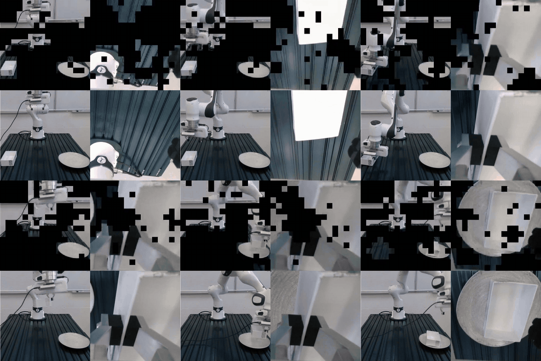
The repository labels this real-robot animation as 2× playback, so visual motion speed is not a latency measurement. The hardware study uses two tasks and 50 rollouts per task and method. On pick, latency changes from 121.13 to 96.90 ms while success changes from 84% to 80%. On pick-and-place, latency changes from 120.01 to 97.77 ms while success changes from 68% to 66%. See the real-robot results.
These measurements support practical deployment, but their scope remains one robot, two tasks, and a particular demonstration setup. They do not establish unchanged success for every small object, camera arrangement, or occlusion pattern. Begin a new deployment with mild pruning, inspect rollout videos, and increase rho between episodes. Separate object-selection failures, approach failures, grasp failures, and placement failures; one aggregate success number can conceal a serious regression in a specific phase.
9. Troubleshooting and a manageable next experiment
- Imports fail: confirm the active conda environment, editable installation, and
PYTHONPATH. A small import check is cheaper than repeatedly loading a 7B model. - Simulator outcomes differ: inspect pinned versions and asset paths. Establish a working baseline before attributing failures to compression.
- GPU memory runs out: inspect competing processes, checkpoint size, and camera configuration. Pruning visual tokens does not guarantee that model weights fit in memory.
- Latency barely improves: check the GPU, CUDA stack, warm-up behavior, system load, and timing scope. Vision encoding or the action head may dominate a different setup.
- Success falls sharply: lower
rho, verify action normalization, and confirm episode resets. Change one factor at a time rather than altering cameras, checkpoint, and pruning together.
After reproducing one suite, expand to all four and sweep a small set of compression targets on a separate validation set. Choose an operating point using the success loss your application can tolerate and the latency actually measured on its hardware. For another perspective on selecting visual tokens, read VLA-ACL and LIBERO token pruning.
FastVLA is useful when you already have a capable VLA policy and want to reduce inference cost without training an additional compressor. The practical lesson is to allocate visual computation according to the current decision, while maintaining a clear baseline that makes the accuracy–latency trade-off measurable.