Why Single-Step Prediction Fails
In Part 2, I introduced Behavioral Cloning — training a policy to predict 1 action per observation. This simple method works for many tasks, but fails catastrophically with complex manipulation tasks. Why?
Problem 1: Temporal Correlation
Robot actions are not independent — action at timestep t strongly depends on actions at t-1, t-2, t-3... When predicting each action individually, the policy loses temporal coherence:
Single-step prediction:
  t=0: move left (correct)
  t=1: move right (noise → wrong direction)
  t=2: move left (correct)
  → Robot shakes, not smooth

Action chunking:
  t=0: predict [left, left, left, left] (entire chunk)
  t=4: predict [down, down, down, down]
  → Robot moves smoothly
Problem 2: Multimodality
Same observation, expert can perform multiple ways. Example: grasping an object from left or right are both valid. Single-step BC with MSE loss will average 2 modes → robot's hand goes straight into the middle (correct mode neither).
Action Chunking with Transformers (ACT) solves both problems. Original paper: Learning Fine-Grained Bimanual Manipulation with Low-Cost Hardware (Zhao et al., RSS 2023).

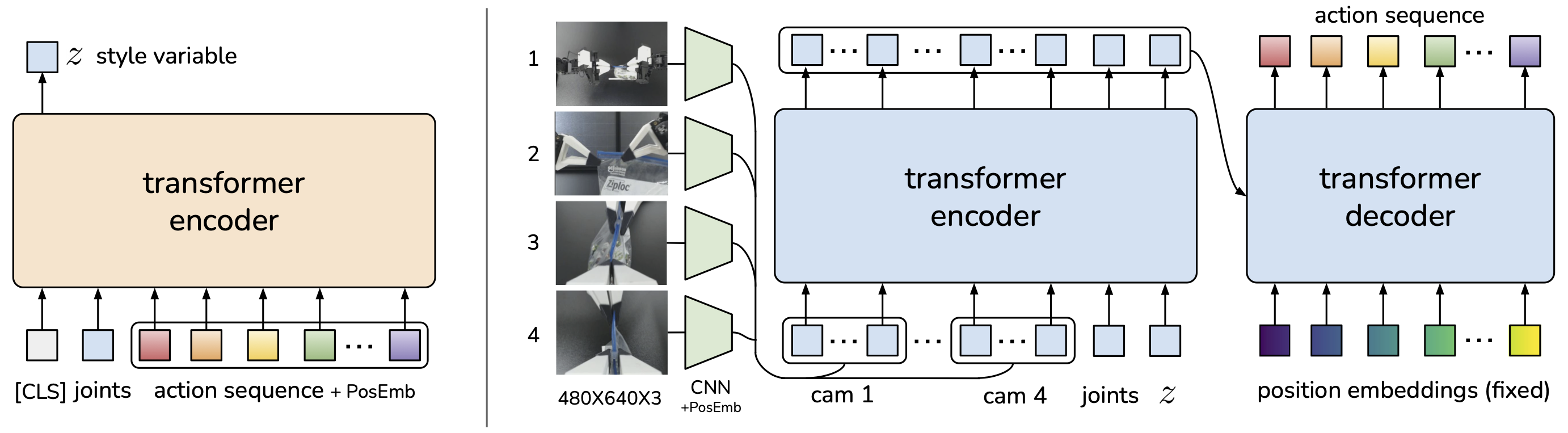
ACT Architecture: Overview
ACT consists of 2 main components:
Training time:
  Observations (images + proprio) ──┐
  Action sequence (ground truth) ───┤
                                    ▼
                              CVAE Encoder
                                    │
                              style variable z
                                    │
                                    ▼
  Observations ─────────────→ Transformer Decoder ──→ Action chunk (k actions)
                                    ▲
                              z (style conditioning)

Inference time:
  Observations ─────────────→ Transformer Decoder ──→ Action chunk
                                    ▲
                              z = 0 (mean of prior)
Why this architecture?
- Action chunking: Predict k actions simultaneously (typically k=100) instead of 1 → solves temporal correlation
- CVAE encoder: Captures multimodality — style variable z encodes "how to do it" (left vs right)
- Transformer decoder: Powerful sequence model, attention between observations and action tokens
CVAE Encoder: Capturing Style
CVAE (Conditional Variational Autoencoder) handles multimodality. Idea: many ways to perform a task, each way is a "style". CVAE encodes style into latent variable z.
Training phase
Input:
  - Observation: camera images + joint positions
  - Action sequence: ground truth actions (k steps)

CVAE Encoder:
  1. Concatenate [CLS token, action tokens] (k+1 tokens)
  2. Cross-attend to observation features
  3. CLS token output → MLP → μ, σ (Gaussian parameters)
  4. Sample z ~ N(μ, σ²)

Loss:
  L = L_reconstruction + β × KL(q(z|o,a) || p(z))

  L_reconstruction = ||predicted_actions - ground_truth_actions||²
  KL regularization: push z distribution near N(0, I)
  β = 10 (in original paper, quite large → force z meaningful)
Inference phase
At deployment, no ground truth actions → don't run encoder. Instead, use z = 0 (mean of prior distribution N(0, I)). This works because:
- KL regularization pushes posterior near prior
- z = 0 gives "average style" — most common behavior in demos
- To get diverse behavior, can sample z ~ N(0, I)
Why not just use Gaussian Mixture Model?
GMM also captures multimodality, but:
- Must choose number of modes K beforehand — don't know how many ways exist
- Doesn't scale to high action dimensions (7D × 100 steps = 700D)
- CVAE learns continuous latent space — smooth interpolation between styles
Transformer Decoder: Generating Action Chunks
Transformer decoder takes observation features and style variable z, generates k sequential actions.
Architecture details
# Simplified ACT decoder architecture
class ACTDecoder(nn.Module):
    def __init__(
        self,
        action_dim=14,        # 7 per arm × 2 arms (bimanual)
        chunk_size=100,       # Predict 100 future actions
        hidden_dim=512,
        n_heads=8,
        n_layers=4,
        latent_dim=32,        # CVAE latent dimension
    ):
        # Observation processing
        self.image_encoder = ResNet18()  # Visual features
        self.proprio_proj = nn.Linear(14, hidden_dim)

        # Style conditioning
        self.style_proj = nn.Linear(latent_dim, hidden_dim)

        # Learnable action queries (like DETR object queries)
        self.action_queries = nn.Embedding(chunk_size, hidden_dim)

        # Transformer decoder layers
        self.decoder = nn.TransformerDecoder(
            nn.TransformerDecoderLayer(
                d_model=hidden_dim,
                nhead=n_heads,
                dim_feedforward=2048,
                batch_first=True,
            ),
            num_layers=n_layers,
        )

        # Action prediction head
        self.action_head = nn.Linear(hidden_dim, action_dim)
Forward pass
1. Process observations:
   - Images → ResNet18 → flatten → visual tokens (49 tokens, 1 token per patch)
   - Joint positions → linear projection → 1 proprio token
   - Style z → linear projection → 1 style token

2. Memory = [visual_tokens, proprio_token, style_token]  (51 tokens)

3. Queries = learnable action_queries  (100 tokens)

4. Transformer Decoder:
   - Self-attention: action queries attend to each other
   - Cross-attention: action queries attend to memory (observations + style)
   - 4 layers

5. Output: 100 action predictions, each 14D vector
   (7D per arm: x, y, z, rx, ry, rz, gripper)
Important point: action queries are learnable — model learns position encoding for each timestep within chunk. Query 0 "knows" it predicts immediate action, query 99 "knows" it predicts far future action.
Temporal Ensembling: Smooth Execution
Action chunking solves temporal correlation, but creates new problem: chunk transitions. When finishing 1 chunk and starting new one, can get "glitch" (discontinuity).
How it works
Instead of executing whole chunk then predicting new one, ACT predicts new chunk every timestep and uses exponential weighting to blend:
Timestep t:
  Chunk predicted at t-2:  [_, _, a_t^(t-2), a_{t+1}^(t-2), ...]
  Chunk predicted at t-1:  [_, a_t^(t-1), a_{t+1}^(t-1), ...]
  Chunk predicted at t:    [a_t^(t), a_{t+1}^(t), ...]

  Action to execute = weighted_average(a_t^(t-2), a_t^(t-1), a_t^(t))

  Weights: w_i = exp(-m × i) where m > 0
  → Most recent chunk has highest weight
  → Older chunks gradually fade in influence
Why exponential weighting?
- Most recent chunk has newest observations → most accurate information → high weight
- Older chunks based on old observations → less relevant but already committed → keep small portion for smoothness
- m (temporal weight) is hyperparameter: large m = reactive (only newest chunk), small m = smooth (blend many chunks)
In original paper, temporal ensembling increases success rate 5-10% on hard tasks — especially important for contact-rich manipulation.

Training Pipeline
Data format (ALOHA)
ACT designed for ALOHA system — 2 robot arms, each 6-DoF + 1 gripper:
# Each episode in dataset
episode = {
    "observations": {
        "images": {
            "cam_high": np.array((T, 480, 640, 3)),   # Top camera
            "cam_left_wrist": np.array((T, 480, 640, 3)),  # Left wrist camera
            "cam_right_wrist": np.array((T, 480, 640, 3)), # Right wrist camera
        },
        "qpos": np.array((T, 14)),  # Joint positions: 7 left + 7 right
        "qvel": np.array((T, 14)),  # Joint velocities
    },
    "actions": np.array((T, 14)),   # Target joint positions
}
Training configuration
# Hyperparameters from paper
config = {
    "chunk_size": 100,        # Predict 100 future actions
    "hidden_dim": 512,
    "n_heads": 8,
    "n_encoder_layers": 4,    # CVAE encoder
    "n_decoder_layers": 7,    # Transformer decoder
    "latent_dim": 32,         # CVAE latent dimension
    "kl_weight": 10,          # β for KL loss
    "lr": 1e-5,
    "batch_size": 8,
    "epochs": 2000,
    "backbone": "resnet18",
    "temporal_agg": True,     # Temporal ensembling
    "temporal_agg_m": 0.01,   # Exponential decay factor
}
Loss function
def compute_loss(model, batch, kl_weight=10):
    """ACT training loss = reconstruction + KL divergence."""
    observations = batch["observations"]
    gt_actions = batch["actions"]  # (B, chunk_size, action_dim)

    # Forward pass — encoder receives both observations and gt_actions
    pred_actions, mu, logvar = model(observations, gt_actions)

    # Reconstruction loss: L1 instead of MSE (robust to outliers)
    l1_loss = F.l1_loss(pred_actions, gt_actions)

    # KL divergence: push posterior near prior N(0, I)
    kl_loss = -0.5 * torch.sum(1 + logvar - mu.pow(2) - logvar.exp())
    kl_loss = kl_loss / (mu.shape[0] * mu.shape[1])  # normalize

    total_loss = l1_loss + kl_weight * kl_loss

    return total_loss, {
        "l1_loss": l1_loss.item(),
        "kl_loss": kl_loss.item(),
        "total_loss": total_loss.item(),
    }
Practical: Train ACT with LeRobot
LeRobot (Hugging Face) is best open-source framework for training and deploying ACT. Wraps entire pipeline into simple CLI commands.
Installation
pip install lerobot
# Or from source for latest features
git clone https://github.com/huggingface/lerobot.git
cd lerobot && pip install -e ".[all]"
Train ACT on ALOHA dataset
# Download dataset and train ACT — 1 command only
lerobot-train \
    --policy.type=act \
    --dataset.repo_id=lerobot/aloha_sim_insertion_human \
    --training.num_epochs=2000 \
    --training.batch_size=8 \
    --policy.chunk_size=100 \
    --policy.n_action_steps=100 \
    --policy.kl_weight=10 \
    --output_dir=outputs/act_insertion
Train on custom dataset
"""
Train ACT on self-collected data with LeRobot.
Requirements: pip install lerobot torch
"""
from lerobot.common.datasets.lerobot_dataset import LeRobotDataset
from lerobot.common.policies.act.modeling_act import ACTPolicy
from lerobot.common.policies.act.configuration_act import ACTConfig

# 1. Load dataset (LeRobot format on HuggingFace Hub)
dataset = LeRobotDataset(
    repo_id="your-username/your-robot-dataset",
    split="train",
)
print(f"Dataset: {len(dataset)} frames, {dataset.num_episodes} episodes")

# 2. Configure ACT policy
config = ACTConfig(
    input_shapes={
        "observation.images.top": [3, 480, 640],
        "observation.state": [14],  # Joint positions
    },
    output_shapes={
        "action": [14],  # Target joint positions
    },
    input_normalization_modes={
        "observation.images.top": "mean_std",
        "observation.state": "mean_std",
    },
    output_normalization_modes={
        "action": "mean_std",
    },
    chunk_size=100,
    n_action_steps=100,
    dim_model=512,
    n_heads=8,
    n_encoder_layers=4,
    n_decoder_layers=7,
    dim_feedforward=2048,
    latent_dim=32,
    use_vae=True,           # Enable CVAE encoder
    kl_weight=10.0,
    temporal_ensemble_coeff=0.01,  # Temporal ensembling
)

# 3. Create policy
policy = ACTPolicy(config=config, dataset_stats=dataset.stats)

# 4. Training loop
import torch
from torch.utils.data import DataLoader

device = torch.device("cuda" if torch.cuda.is_available() else "cpu")
policy = policy.to(device)
optimizer = torch.optim.AdamW(policy.parameters(), lr=1e-5, weight_decay=1e-4)

dataloader = DataLoader(dataset, batch_size=8, shuffle=True, num_workers=4)

for epoch in range(2000):
    epoch_loss = 0
    for batch in dataloader:
        batch = {k: v.to(device) for k, v in batch.items()}
        output = policy.forward(batch)
        loss = output["loss"]

        optimizer.zero_grad()
        loss.backward()
        torch.nn.utils.clip_grad_norm_(policy.parameters(), 10.0)
        optimizer.step()

        epoch_loss += loss.item()

    if epoch % 100 == 0:
        avg_loss = epoch_loss / len(dataloader)
        print(f"Epoch {epoch}: loss={avg_loss:.6f}")

# 5. Save policy
policy.save_pretrained("outputs/act_custom/")
print("Training complete!")
Evaluate and deploy
"""Run ACT policy on robot or simulation."""
from lerobot.common.policies.act.modeling_act import ACTPolicy

# Load trained policy
policy = ACTPolicy.from_pretrained("outputs/act_custom/")
policy.eval()

# Inference loop with temporal ensembling
action_queue = []  # Buffer for temporal ensembling

for step in range(max_steps):
    observation = robot.get_observation()

    # Policy predict chunk of actions
    with torch.no_grad():
        action_chunk = policy.select_action(observation)
        # action_chunk shape: (chunk_size, action_dim)

    # Temporal ensembling
    action_queue.append(action_chunk)
    if len(action_queue) > max_queue_len:
        action_queue.pop(0)

    # Weighted average
    weights = [
        np.exp(-0.01 * i)
        for i in range(len(action_queue) - 1, -1, -1)
    ]
    weights = np.array(weights) / sum(weights)

    action = sum(w * q[len(action_queue) - 1 - i]
                 for i, (w, q) in enumerate(zip(weights, action_queue)))

    robot.execute_action(action)
Results and Comparison
ACT achieves impressive results on ALOHA bimanual tasks — tasks that standard BC barely solves:
| Task | BC (single-step) | ACT (no temporal agg) | ACT (full) |
|---|---|---|---|
| Slot insertion | 10% | 80% | 96% |
| Transfer cube | 2% | 72% | 90% |
| Thread zip tie | 0% | 40% | 52% |
| Open cup | 0% | 55% | 68% |
Notes:
- BC single-step nearly completely fails on bimanual tasks — distribution shift too severe
- Action chunking alone (no temporal ensembling) already boosts performance significantly
- Temporal ensembling adds 5-16% success rate depending on task
Comparison with other methods
| Method | Demos needed | Train time | Bimanual | Fine-grained |
|---|---|---|---|---|
| BC (MLP) | 50 | 10 min | Poor | Poor |
| BC (Transformer) | 50 | 30 min | Average | Average |
| Diffusion Policy | 50 | 2 hours | Good | Good |
| ACT | 50 | 1 hour | Very good | Very good |
| ACT + Diffusion | 50 | 3 hours | Very good | Very good |
ACT balances performance and training cost well. Diffusion Policy may be better for some tasks, but trains and infers slower.
Key Takeaways
- Action chunking solves temporal correlation — predict k actions together maintains coherence
- CVAE encoder captures multimodality — style variable z encodes "how to do it"
- Temporal ensembling for smooth execution — blend multiple chunks with exponential weighting
- 50 demonstrations sufficient for many manipulation tasks — don't need thousands of demos
- LeRobot is fastest way to start — download dataset, train, deploy in one day
Next Steps
ACT is state-of-the-art for imitation learning from demonstrations. But if you want robot to understand language instructions ("pick up the red cup"), you need foundation models — see Foundation Models for Robot: RT-2, Octo, OpenVLA in Practice to understand how to combine vision, language, and action in one model.
Related Posts
- RL for Robotics: PPO, SAC and How to Choose Algorithm — Part 1: RL foundation for robots
- Imitation Learning: BC, DAgger and DAPG for Robot — Part 2: Imitation learning basics
- Foundation Models for Robot: RT-2, Octo, OpenVLA in Practice — Next step: vision-language-action models
- Sim-to-Real Transfer: Train in Simulation, Run on Real Robot — Transfer ACT policy from sim to real