What is SLAM and why does it matter?
SLAM (Simultaneous Localization and Mapping) is the most fundamental problem in robot navigation: the robot simultaneously builds a map of the environment while determining its own location on that map. This is the classic "chicken and egg" problem: to localize you need a map, but to build a map you need to know your position.
Every AMR (Autonomous Mobile Robot) operating in factories, warehouses, or outdoors needs SLAM. Without SLAM, a robot is just a remotely controlled vehicle.
In this article, I'll guide you from fundamental theory (EKF-SLAM, particle filters) to modern frameworks (ORB-SLAM3, Cartographer, LIO-SAM), and help you choose the right method for your use case.

Theoretical Foundation of SLAM
SLAM as a Probabilistic Problem
SLAM can be modeled as a Bayesian estimation problem. At each timestep t, the robot needs to estimate:
- State: robot position and orientation (x, y, theta)
- Map: landmark positions or occupancy grid
- Observations: sensor data (LiDAR scans, camera frames)
- Controls: control commands (velocity, steering angle)
Objective: find probability distribution P(x_t, m | z_{1:t}, u_{1:t}) — the probability of robot location and map given all observations and controls from start to time t.
EKF-SLAM — Extended Kalman Filter
EKF-SLAM is the most classical method, using Extended Kalman Filter to simultaneously estimate robot position and landmark positions.
How it works:
- Predict: use motion model to predict new robot pose
- Update: when observing landmarks, update both robot pose and landmark positions
State vector contains robot pose (3 values) + all landmark positions (2N values for N landmarks). Covariance matrix has size (3+2N) x (3+2N).
# EKF-SLAM simplified pseudocode
def ekf_slam_predict(mu, sigma, u):
    # Motion model: predict new robot pose
    mu_bar = motion_model(mu, u)
    G = jacobian_motion(mu, u)
    sigma_bar = G @ sigma @ G.T + R  # R: motion noise
    return mu_bar, sigma_bar

def ekf_slam_update(mu_bar, sigma_bar, z, landmark_id):
    # Observation model: update with landmark measurement
    z_hat = observation_model(mu_bar, landmark_id)
    H = jacobian_observation(mu_bar, landmark_id)
    K = sigma_bar @ H.T @ inv(H @ sigma_bar @ H.T + Q)
    mu = mu_bar + K @ (z - z_hat)
    sigma = (I - K @ H) @ sigma_bar
    return mu, sigma
Advantages: solid theory, easy to understand, convergent with small number of landmarks.
Disadvantages: O(N^2) complexity with N landmarks -- doesn't scale for large maps. Gaussian assumption doesn't fit complex environments well.
Particle Filter SLAM (FastSLAM)
FastSLAM (Montemerlo et al., 2002) solves scalability issues by using particle filters for robot pose and separate EKF for each landmark in each particle.
How it works:
- Each particle represents a hypothesis about the robot's trajectory
- Each particle has its own EKF for each landmark
- Resampling selects particles with highest probability
Complexity: O(M * N) with M particles and N landmarks -- much better than EKF-SLAM.
FastSLAM 2.0 further improves by using the latest observation to sample particles, reducing number of particles needed.
LiDAR SLAM — Industrial Standard
Google Cartographer
Cartographer is a 2D/3D SLAM system developed by Google, open-source since 2016. It's one of the most widely used LiDAR SLAM systems in industry.
Architecture:
- Local SLAM (Frontend): scan matching using Ceres Solver (nonlinear least squares), creating submaps from consecutive LiDAR scans
- Global SLAM (Backend): pose graph optimization for closing loop closures, using branch-and-bound scan matching
Strengths:
- Real-time 2D SLAM on standard hardware
- 3D SLAM with multi-LiDAR setup
- Good integration with ROS 1 and ROS 2
- Pure LiDAR, no need for IMU (though IMU improves accuracy)
# Run Cartographer with ROS 2
ros2 launch cartographer_ros cartographer.launch.py \
  use_sim_time:=true
LIO-SAM — LiDAR-Inertial Odometry via Smoothing and Mapping
LIO-SAM (Shan et al., 2020) is a framework for tightly-coupled LiDAR-inertial SLAM using factor graph optimization. Original paper: arXiv:2007.00258.
Architecture:
- IMU pre-integration factor: computes relative motion between LiDAR scans
- LiDAR odometry factor: point-to-plane and point-to-edge matching
- GPS factor (optional): for outdoor navigation
- Loop closure factor: detects and corrects drift
Why LIO-SAM is powerful:
- IMU helps de-skew LiDAR point cloud (critical when robot moves fast)
- Factor graph allows adding multiple information sources (GPS, wheel odometry)
- Keyframe-based: only stores important frames, reduces memory
# LIO-SAM config (params.yaml)
lio_sam:
  pointCloudTopic: "points_raw"
  imuTopic: "imu_correct"
  gpsTopic: "odometry/gps"

  # Lidar sensor
  sensor: velodyne  # velodyne, ouster, livox
  N_SCAN: 16
  Horizon_SCAN: 1800

  # IMU
  imuAccNoise: 3.9939570888238808e-03
  imuGyrNoise: 1.5636343949698187e-03

Visual SLAM — Camera is Enough
ORB-SLAM3
ORB-SLAM3 (Campos et al., 2021) is the most comprehensive Visual-Inertial SLAM system to date. Paper: arXiv:2007.11898.
Supports:
- Monocular: 1 camera (has scale ambiguity)
- Stereo: 2 cameras (full metric scale)
- RGB-D: depth camera (like Intel RealSense)
- Visual-Inertial: camera + IMU (monocular-inertial or stereo-inertial)
Pipeline:
- Tracking: extract ORB features, match with local map, estimate camera pose
- Local Mapping: triangulate new map points, local bundle adjustment
- Loop Closing: DBoW2 bag-of-words for place recognition, pose graph optimization
- Multi-map: manage multiple maps when tracking fails, merge when reconnecting
Strengths: accurate, robust, supports many camera types, multi-map system.
Weaknesses: needs texture-rich environment (fails in white corridors), higher computational cost than LiDAR SLAM.
// ORB-SLAM3 basic usage
ORB_SLAM3::System SLAM(
    vocab_path,           // ORB vocabulary
    settings_path,        // Camera + ORB params
    ORB_SLAM3::System::RGBD,  // Sensor type
    true                  // Visualization
);

// Process each frame
cv::Mat Tcw = SLAM.TrackRGBD(imRGB, imD, timestamp);
RTAB-Map — Real-Time Appearance-Based Mapping
RTAB-Map is the Visual SLAM best integrated with ROS 2. Supports many sensor types and has smart memory management.
Highlights:
- Multi-session mapping: save and load maps between runs
- Support for 2D occupancy grid (for navigation) and 3D point cloud
- Graph-based SLAM with visual loop closure
- ROS 2 package ready to use
Comprehensive Comparison Table
| Method | Sensor | Accuracy | Speed | Outdoor | Indoor | Scale |
|---|---|---|---|---|---|---|
| EKF-SLAM | Any | Medium | Fast | Yes | Yes | Small (<100 landmarks) |
| FastSLAM | Any | High | Medium | Yes | Yes | Medium |
| Cartographer | LiDAR | High | Real-time | Limited | Best | Large |
| LIO-SAM | LiDAR+IMU | Very high | Real-time | Good | Good | Very large |
| ORB-SLAM3 | Camera(+IMU) | High | Real-time | Yes | Good | Medium |
| RTAB-Map | Camera/LiDAR | High | Real-time | Yes | Good | Large |
When to use which method?
Choose LiDAR SLAM (Cartographer / LIO-SAM) when:
- Environment is structured with fixed walls (factories, warehouses)
- Need high accuracy and reliability for production
- Robot moves at high speed (LIO-SAM with IMU de-skew)
- Budget allows LiDAR purchase (from $200 for 2D to $5,000+ for 3D)
Choose Visual SLAM (ORB-SLAM3 / RTAB-Map) when:
- Limited budget -- camera is much cheaper than LiDAR
- Need semantic information (object recognition, text)
- Environment has rich texture (not white corridors)
- Combining with other computer vision tasks
Choose Hybrid (Visual-Inertial or LiDAR-Inertial) when:
- Need highest reliability -- sensor fusion increases robustness
- Environment changes frequently (lighting, dynamic objects)
- Robot operates both indoors and outdoors
Emerging Trend: Learning-based SLAM
Traditional SLAM methods rely on geometric constraints. But deep learning is changing the game:
- DROID-SLAM (Teed & Deng, 2021): end-to-end differentiable SLAM, surpassing ORB-SLAM3 accuracy on many benchmarks. Paper: arXiv:2108.10869.
- Gaussian Splatting SLAM: uses 3D Gaussian Splatting to create photorealistic maps, enabling novel view synthesis.
- Foundation model-based place recognition: uses CLIP, DINOv2 for better loop closure than traditional bag-of-words.
We'll dive deeper into learning-based navigation in Part 3 of this series.
Next in the series
This is Part 1 of the Modern Navigation series. In upcoming articles:
- Part 2: ROS 2 Nav2: Complete Navigation for AMR -- Nav2 stack, path planning, behavior trees
- Part 3: Learning-based Navigation: GNM, ViNT and NoMaD -- Foundation models for robot navigation
- Part 4: Vision-Language Navigation: Robot follows instructions -- VLN task and LLM-based planning
- Part 5: Outdoor Navigation and Multi-Robot Coordination -- GPS-denied nav, MAPF algorithms
Related articles
- ROS 2 Nav2 deep-dive -- Detailed guide to Nav2 stack in ROS 2
- LiDAR 3D Mapping -- LiDAR technology and applications in robotics
- Simulation for Robotics: MuJoCo vs Isaac Sim vs Gazebo -- Test SLAM algorithms in simulation
- Edge AI with NVIDIA Jetson -- Deploy SLAM on embedded hardware