What is Inverse Kinematics and Why Does It Matter?
Inverse Kinematics (IK) for 6-DOF robot arms is a core robotics problem: given a desired end-effector position and orientation, find the corresponding joint angles. If you've ever programmed a robot to grasp an object, you know that humans think in Cartesian coordinates ("move the hand to point x, y, z"), but robots need individual joint angles. IK is the bridge between these two worlds.
This post covers the theory from Denavit-Hartenberg (DH) parameters, through forward kinematics, to a complete numerical IK solver in Python. The code is self-contained — requiring only NumPy and Matplotlib, no specialized robotics libraries.

Denavit-Hartenberg Convention
Why Do We Need DH Parameters?
Each robot arm has different joint and link configurations. The DH convention provides a standardized method to describe the geometric relationships between successive joints using exactly 4 parameters per joint:
| Parameter | Symbol | Meaning |
|---|---|---|
| Link length | a_i | Distance between z_{i-1} and z_i axes along x_i axis |
| Link twist | alpha_i | Rotation angle from z_{i-1} to z_i around x_i axis |
| Link offset | d_i | Distance along z_{i-1} axis |
| Joint angle | theta_i | Rotation around z_{i-1} axis (variable for revolute joint) |
DH Transformation Matrix
Each set of DH parameters produces a 4x4 homogeneous transformation matrix:
import numpy as np

def dh_matrix(theta, d, a, alpha):
    """
    Create DH transformation matrix 4x4.
    theta: joint angle (rad)
    d: link offset
    a: link length
    alpha: link twist (rad)
    """
    ct, st = np.cos(theta), np.sin(theta)
    ca, sa = np.cos(alpha), np.sin(alpha)

    return np.array([
        [ct, -st * ca,  st * sa, a * ct],
        [st,  ct * ca, -ct * sa, a * st],
        [0,   sa,       ca,      d     ],
        [0,   0,        0,       1     ]
    ])
This matrix encodes both rotation and translation. Multiplying 6 matrices together gives us forward kinematics — the end-effector position and orientation from joint angles.
Forward Kinematics for 6-DOF Robots
Example: Puma 560-Style Robot
Below is a sample DH parameters table for a 6-revolute-joint robot (units: meters, radians):
# DH Parameters for anthropomorphic 6-DOF robot
# Each row: [a, alpha, d, theta_offset]
# Actual theta = theta_variable + theta_offset
DH_PARAMS = [
    # a      alpha        d      theta_offset
    [0.0,    np.pi/2,     0.4,   0.0],   # Joint 1 (base rotation)
    [0.25,   0.0,         0.0,   0.0],   # Joint 2 (shoulder)
    [0.025,  np.pi/2,     0.0,   0.0],   # Joint 3 (elbow)
    [0.0,   -np.pi/2,     0.28,  0.0],   # Joint 4 (wrist roll)
    [0.0,    np.pi/2,     0.0,   0.0],   # Joint 5 (wrist pitch)
    [0.0,    0.0,         0.1,   0.0],   # Joint 6 (wrist yaw)
]

def forward_kinematics(joint_angles, dh_params=DH_PARAMS):
    """
    Compute end-effector position and orientation from joint angles.
    Returns 4x4 matrix (rotation + position).
    """
    T = np.eye(4)
    for i, (a, alpha, d, offset) in enumerate(dh_params):
        theta = joint_angles[i] + offset
        T = T @ dh_matrix(theta, d, a, alpha)
    return T

# Test: all joints at zero position
q_home = np.zeros(6)
T_home = forward_kinematics(q_home)
position = T_home[:3, 3]
print(f"Home position: x={position[0]:.3f}, y={position[1]:.3f}, z={position[2]:.3f}")
Extracting Position and Orientation
def extract_pose(T):
    """Extract position (xyz) and rotation matrix from 4x4 matrix T."""
    position = T[:3, 3]
    rotation = T[:3, :3]
    return position, rotation

def rotation_to_euler(R):
    """Convert rotation matrix to Euler angles (ZYX convention)."""
    sy = np.sqrt(R[0, 0]**2 + R[1, 0]**2)
    singular = sy < 1e-6

    if not singular:
        roll  = np.arctan2(R[2, 1], R[2, 2])
        pitch = np.arctan2(-R[2, 0], sy)
        yaw   = np.arctan2(R[1, 0], R[0, 0])
    else:
        roll  = np.arctan2(-R[1, 2], R[1, 1])
        pitch = np.arctan2(-R[2, 0], sy)
        yaw   = 0.0

    return np.array([roll, pitch, yaw])
Jacobian Matrix — The Key to Numerical IK
What is the Jacobian?
The Jacobian matrix J describes the differential relationship between joint velocities and end-effector velocities:
v = J(q) * dq
Where v is a 6D vector (3 linear + 3 angular velocities) and q is the joint angle vector. For numerical IK, the Jacobian tells us: "if I want the end-effector to move delta_x, how much do I change the joint angles?"
Computing the Jacobian via Finite Differences
The simplest and most robust method is finite differences:
def compute_jacobian(joint_angles, dh_params=DH_PARAMS, delta=1e-6):
    """
    Compute numerical Jacobian (6x6) via finite differences.
    Rows 0-2: linear velocity (dx, dy, dz)
    Rows 3-5: angular velocity (drx, dry, drz)
    """
    n_joints = len(joint_angles)
    J = np.zeros((6, n_joints))

    T_current = forward_kinematics(joint_angles, dh_params)
    pos_current, R_current = extract_pose(T_current)
    euler_current = rotation_to_euler(R_current)

    for i in range(n_joints):
        q_perturbed = joint_angles.copy()
        q_perturbed[i] += delta

        T_perturbed = forward_kinematics(q_perturbed, dh_params)
        pos_perturbed, R_perturbed = extract_pose(T_perturbed)
        euler_perturbed = rotation_to_euler(R_perturbed)

        # Linear velocity columns
        J[:3, i] = (pos_perturbed - pos_current) / delta
        # Angular velocity columns
        J[3:, i] = (euler_perturbed - euler_current) / delta

    return J

Numerical IK Solver: Newton-Raphson Method
The Algorithm
Core idea: iteratively compute error between current and desired pose, then use pseudo-inverse Jacobian to update joint angles:
while |error| > tolerance:
    error = target_pose - current_pose
    dq = J_pinv * error
    q = q + dq
Full Implementation
def pose_error(T_current, T_target):
    """
    Compute 6D error between current and target pose.
    Returns: [dx, dy, dz, drx, dry, drz]
    """
    pos_err = T_target[:3, 3] - T_current[:3, 3]

    R_current = T_current[:3, :3]
    R_target = T_target[:3, :3]
    R_err = R_target @ R_current.T

    # Extract rotation error as axis-angle
    angle = np.arccos(np.clip((np.trace(R_err) - 1) / 2, -1, 1))
    if angle < 1e-6:
        rot_err = np.zeros(3)
    else:
        rot_err = angle / (2 * np.sin(angle)) * np.array([
            R_err[2, 1] - R_err[1, 2],
            R_err[0, 2] - R_err[2, 0],
            R_err[1, 0] - R_err[0, 1]
        ])

    return np.concatenate([pos_err, rot_err])


def inverse_kinematics(T_target, q_init=None, dh_params=DH_PARAMS,
                        max_iter=200, pos_tol=1e-4, rot_tol=1e-3,
                        damping=0.1):
    """
    Numerical IK solver using Damped Least Squares (Levenberg-Marquardt).

    Args:
        T_target: 4x4 target matrix
        q_init: joint angle initialization (None = zeros)
        max_iter: maximum iterations
        pos_tol: position error tolerance (meters)
        rot_tol: orientation error tolerance (rad)
        damping: damping coefficient lambda (avoid singularity)

    Returns:
        q_solution: solution joint angles
        success: True if converged
        iterations: actual iterations taken
    """
    n_joints = len(dh_params)
    q = q_init.copy() if q_init is not None else np.zeros(n_joints)

    for iteration in range(max_iter):
        T_current = forward_kinematics(q, dh_params)
        error = pose_error(T_current, T_target)

        pos_err_norm = np.linalg.norm(error[:3])
        rot_err_norm = np.linalg.norm(error[3:])

        # Check convergence
        if pos_err_norm < pos_tol and rot_err_norm < rot_tol:
            return q, True, iteration

        # Compute Jacobian and damped pseudo-inverse
        J = compute_jacobian(q, dh_params)
        # Damped Least Squares: dq = J^T (J J^T + lambda^2 I)^(-1) * error
        JJT = J @ J.T
        dq = J.T @ np.linalg.solve(
            JJT + damping**2 * np.eye(6), error
        )

        q = q + dq

        # Clamp joint angles to [-pi, pi]
        q = np.mod(q + np.pi, 2 * np.pi) - np.pi

    return q, False, max_iter


# === EXAMPLE USAGE ===

# Step 1: Forward kinematics to create target pose
q_desired = np.array([0.3, -0.5, 0.8, 0.1, -0.3, 0.6])
T_target = forward_kinematics(q_desired)

print("Target position:", T_target[:3, 3])
print("Target angles (ground truth):", np.degrees(q_desired))

# Step 2: Solve IK from different initial guess
q_init = np.array([0.0, 0.0, 0.0, 0.0, 0.0, 0.0])
q_solution, success, iters = inverse_kinematics(T_target, q_init)

print(f"\nIK {'converged' if success else 'FAILED'} after {iters} iterations")
print(f"Solution angles: {np.degrees(q_solution).round(2)}")

# Verify
T_result = forward_kinematics(q_solution)
pos_error = np.linalg.norm(T_target[:3, 3] - T_result[:3, 3])
print(f"Position error: {pos_error*1000:.3f} mm")
Damped Least Squares vs Pure Pseudo-Inverse
The Singularity Problem
When a robot approaches a singularity (e.g., two wrist joints aligned), the Jacobian becomes nearly singular, and pseudo-inverse produces extremely large values causing uncontrolled robot motion.
Damped Least Squares (also called Levenberg-Marquardt) adds a damping coefficient lambda:
dq = J^T (J J^T + lambda^2 I)^(-1) * error
When lambda = 0, we have pure pseudo-inverse. When lambda is large, motion is slower but stable near singularities. In practice, lambda = 0.01 - 0.5 works well for most robots.
Adaptive Damping
An advanced technique is to adjust lambda based on distance to singularity:
def adaptive_damping(J, lambda_min=0.01, lambda_max=0.5):
    """Increase damping when near singularity."""
    # Manipulability measure
    w = np.sqrt(max(np.linalg.det(J @ J.T), 0))
    # Threshold
    w_threshold = 0.05
    if w < w_threshold:
        ratio = 1.0 - (w / w_threshold)**2
        return lambda_min + ratio * (lambda_max - lambda_min)
    return lambda_min
Practical Tips When Implementing IK
1. Multiple Solutions
A 6-DOF robot typically has up to 8 solutions for the same target pose. The initial guess determines which solution you get. In real applications, choose the solution closest to the current configuration to minimize joint motion:
def best_ik_solution(T_target, q_current, n_trials=10):
    """Try multiple initial guesses, select closest solution."""
    best_q = None
    best_dist = float('inf')

    for _ in range(n_trials):
        q_init = q_current + np.random.uniform(-0.5, 0.5, 6)
        q_sol, success, _ = inverse_kinematics(T_target, q_init)
        if success:
            dist = np.linalg.norm(q_sol - q_current)
            if dist < best_dist:
                best_dist = dist
                best_q = q_sol

    return best_q
2. Joint Limits
Real robots have joint angle limits. Add clamping after each iteration:
JOINT_LIMITS = [
    (-np.pi, np.pi),       # Joint 1
    (-np.pi/2, np.pi/2),   # Joint 2
    (-np.pi*3/4, np.pi*3/4), # Joint 3
    (-np.pi, np.pi),       # Joint 4
    (-np.pi/2, np.pi/2),   # Joint 5
    (-np.pi, np.pi),       # Joint 6
]

def clamp_joints(q, limits=JOINT_LIMITS):
    return np.array([
        np.clip(q[i], limits[i][0], limits[i][1])
        for i in range(len(q))
    ])
3. Workspace Check
Before running IK, verify the target lies within workspace:
def in_workspace(T_target, dh_params=DH_PARAMS):
    """Quick check if target is reachable."""
    pos = T_target[:3, 3]
    dist = np.linalg.norm(pos)
    # Sum of all link lengths
    max_reach = sum(
        np.sqrt(p[0]**2 + p[2]**2) for p in dh_params
    )
    return dist <= max_reach * 0.95  # 95% safety margin
3D Visualization with Matplotlib
import matplotlib.pyplot as plt
from mpl_toolkits.mplot3d import Axes3D

def plot_robot(joint_angles, dh_params=DH_PARAMS, ax=None):
    """Plot 3D robot arm from joint angles."""
    if ax is None:
        fig = plt.figure(figsize=(10, 8))
        ax = fig.add_subplot(111, projection='3d')

    positions = [np.array([0, 0, 0])]
    T = np.eye(4)

    for i, (a, alpha, d, offset) in enumerate(dh_params):
        theta = joint_angles[i] + offset
        T = T @ dh_matrix(theta, d, a, alpha)
        positions.append(T[:3, 3].copy())

    positions = np.array(positions)
    ax.plot(positions[:, 0], positions[:, 1], positions[:, 2],
            'o-', linewidth=3, markersize=8, color='steelblue')
    ax.scatter(*positions[-1], color='red', s=100, zorder=5,
               label='End-effector')
    ax.scatter(*positions[0], color='green', s=100, zorder=5,
               label='Base')

    ax.set_xlabel('X (m)')
    ax.set_ylabel('Y (m)')
    ax.set_zlabel('Z (m)')
    ax.legend()
    ax.set_title('Robot Arm Configuration')
    plt.tight_layout()
    return ax

# Plot home configuration and IK solution
fig, (ax1, ax2) = plt.subplots(1, 2, figsize=(16, 7),
                                subplot_kw={'projection': '3d'})
plot_robot(np.zeros(6), ax=ax1)
ax1.set_title('Home Configuration')

plot_robot(q_solution, ax=ax2)
ax2.set_title('IK Solution')
plt.savefig('robot_ik_comparison.png', dpi=150)
plt.show()

Next Steps
The code in this post is self-contained — requiring only NumPy and Matplotlib. You can extend it further:
- Trajectory planning: Interpolate between multiple IK points using cubic splines
- Collision avoidance: Integrate with MoveIt2 in ROS 2
- Real-time control: Send joint angles via Serial/CAN bus to motor drivers
If you're new to Python for robotics, read Robot Control Programming with Python to understand GPIO, PID, and computer vision fundamentals.