Have you ever wondered why humans walk effortlessly without conscious thought, while humanoid robots struggle to maintain balance? The answer lies in the staggering complexity of bipedal locomotion — and Reinforcement Learning (RL) is becoming the most powerful tool to tackle it.
In this first post of the RL Humanoid Locomotion series, we will lay a solid foundation: understand why humanoid locomotion is hard, formulate the problem as an MDP, and set up the training environment with Isaac Lab.
Why Humanoid Locomotion Is Extremely Hard
Underactuation — Fewer Actuators Than Degrees of Freedom
A humanoid robot is an underactuated system — meaning it has fewer actuators than the degrees of freedom (DOF) it needs to control. When the robot stands on one leg (single support phase), that leg must control the entire body. But foot-ground contact is unilateral — the robot can only push the ground, never pull it. This creates friction cone constraints that any controller must respect.
High Degrees of Freedom
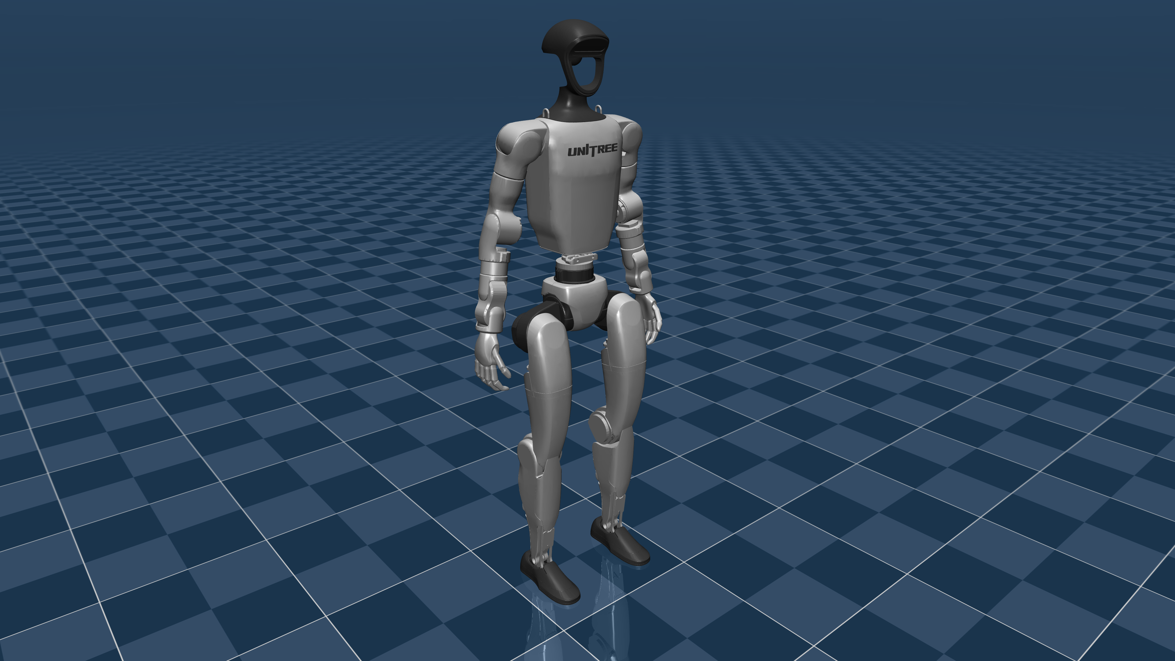
A humanoid like the Unitree G1 has 23 DOF, while the H1 has 19 DOF for legs alone. Compared to a quadruped (12 DOF) or wheeled robot (2-4 DOF), the state and action spaces are orders of magnitude larger:
| Robot | DOF | Observation dim | Action dim |
|---|---|---|---|
| Wheeled robot | 2 | ~10 | 2 |
| Quadruped (Go2) | 12 | ~48 | 12 |
| Humanoid G1 | 23 | ~70+ | 23 |
| Humanoid H1 | 19 | ~60+ | 19 |
Balance and ZMP
The Zero Moment Point (ZMP) is a core concept: the robot is only stable when the ZMP lies within the support polygon (foot contact area). During bipedal walking, the support polygon changes continuously, alternating between double support (both feet) and single support (one foot). During single support, the polygon is tiny — roughly 25x15 cm — making the robot extremely vulnerable to falling.

Why RL Outperforms Traditional Control
Traditional methods (ZMP-based, model predictive control) require an accurate dynamics model and solve optimization problems online. However:
- Models are never perfect (friction, backlash, flexibility)
- Real-time optimization is computationally expensive
- Difficult to generalize to different terrains
RL takes a different approach: learn a policy directly from interactions with a simulator, without requiring an accurate model. The policy naturally learns to handle uncertainty through domain randomization.
If you are new to RL, check out RL Basics for Robotics before continuing.
MDP Formulation for Bipedal Walking
Markov Decision Process
The locomotion problem is formulated as an MDP tuple $(S, A, T, R, \gamma)$:
- State $S$: Complete state of the robot and environment
- Action $A$: Control commands sent to actuators
- Transition $T$: Simulator dynamics (MuJoCo/Isaac Sim)
- Reward $R$: Function evaluating locomotion quality
- Discount $\gamma$: Typically 0.99 for locomotion tasks
Observation Space — What Does the Robot "See"?
The observation is the information the policy receives each timestep. Designing a good observation space is make-or-break:
import torch
import numpy as np

class HumanoidObservation:
    """Observation space for humanoid locomotion."""

    def __init__(self, num_joints=23):
        self.num_joints = num_joints

    def compute_observation(self, robot_state, command):
        """
        Compute observation vector from robot state.

        Returns:
            obs: tensor of shape (obs_dim,)
        """
        obs_components = []

        # 1. Base angular velocity (3D) - from IMU gyroscope
        # Robot needs to know how it is rotating
        base_ang_vel = robot_state["base_angular_velocity"]  # (3,)
        obs_components.append(base_ang_vel)

        # 2. Projected gravity (3D) - gravity direction in robot frame
        # Most important for balance!
        projected_gravity = robot_state["projected_gravity"]  # (3,)
        obs_components.append(projected_gravity)

        # 3. Velocity command (3D) - desired velocity [vx, vy, yaw_rate]
        velocity_command = command["velocity"]  # (3,)
        obs_components.append(velocity_command)

        # 4. Joint positions relative to default (num_joints,)
        # Deviation from default standing pose
        joint_pos_error = (
            robot_state["joint_positions"]
            - robot_state["default_joint_positions"]
        )
        obs_components.append(joint_pos_error)

        # 5. Joint velocities (num_joints,)
        joint_vel = robot_state["joint_velocities"]
        obs_components.append(joint_vel)

        # 6. Previous actions (num_joints,) - previous action
        # Helps policy be smoother, avoids jerkiness
        prev_actions = robot_state["previous_actions"]
        obs_components.append(prev_actions)

        # Concatenate all components
        obs = np.concatenate(obs_components)
        # Total dim: 3 + 3 + 3 + 23 + 23 + 23 = 78 for G1
        return obs
Why is projected gravity the most important? Because it tells the policy how the robot is tilting relative to vertical. Without this information, the robot cannot balance.
Action Space — How Does the Robot Control Itself?
The action space is typically joint position targets — desired angular positions for each joint. A low-level PD controller generates torques for tracking:
class HumanoidActionSpace:
    """Action space: joint position targets + PD control."""

    def __init__(self, num_joints=23):
        self.num_joints = num_joints
        # PD gains for each joint
        self.kp = np.array([
            # Hip (3 DOF each side): higher due to heavy load
            200, 200, 200,  # left hip
            200, 200, 200,  # right hip
            # Knee (1 DOF each side)
            250, 250,
            # Ankle (2 DOF each side)
            40, 40, 40, 40,
            # Torso
            300,
            # Shoulder (3 DOF each side)
            100, 100, 100,
            100, 100, 100,
            # Elbow
            50, 50,
            # Wrist
            20, 20,
        ])
        self.kd = self.kp * 0.05  # Kd = 5% of Kp

    def apply_action(self, action, current_pos, current_vel):
        """
        Convert action (position targets) to torque.

        action: (num_joints,) - scaled position offsets
        """
        # Scale action from [-1, 1] to radian offset
        action_scale = 0.25  # max ±0.25 rad
        target_pos = current_pos + action * action_scale

        # PD control
        torque = self.kp * (target_pos - current_pos) - self.kd * current_vel

        # Clip torque to motor limits
        torque = np.clip(torque, -100, 100)  # Nm
        return torque
Choosing a Simulator: Isaac Lab vs MuJoCo
The choice of simulator directly impacts training speed and sim-to-real transfer quality.
| Criterion | Isaac Lab (NVIDIA) | MuJoCo (DeepMind) |
|---|---|---|
| GPU parallelization | Thousands of envs on GPU | CPU-based (MJX for GPU is new) |
| Training speed | Very fast (~1h for walking) | 10-100x slower |
| Contact physics | Good, GPU-accelerated | Excellent, most accurate |
| Sim-to-real gap | Small with domain rand | Very small |
| Community | Growing rapidly | Mature, many papers |
| Hardware requirements | RTX 3090+ (CUDA) | Any CPU/GPU |
| Best for | Fast training, massively parallel | Research, prototyping |
Recommendation: Use Isaac Lab for training (fast), MuJoCo for debugging and visualization. Many top papers use both.
For detailed Isaac Lab coverage, see Isaac Lab: GPU-Accelerated Robot Simulation.

Setting Up Isaac Lab Environment for Humanoid
Installing Isaac Lab
# Clone Isaac Lab
git clone https://github.com/isaac-sim/IsaacLab.git
cd IsaacLab

# Create conda environment
conda create -n isaaclab python=3.10 -y
conda activate isaaclab

# Install Isaac Sim (requires NVIDIA GPU)
pip install isaacsim-rl isaacsim-replicator isaacsim-extscache-physics \
    isaacsim-extscache-kit-sdk isaacsim-extscache-kit \
    isaacsim-app --extra-index-url https://pypi.nvidia.com

# Install Isaac Lab
pip install -e .
Installing Humanoid-Gym
Humanoid-Gym is a specialized framework for humanoid locomotion built on Isaac Lab:
# Clone Humanoid-Gym
git clone https://github.com/roboterax/humanoid-gym.git
cd humanoid-gym

# Install dependencies
pip install -e .
Loading Unitree G1 in MuJoCo
Start with MuJoCo to understand the robot model before moving to Isaac Lab:
import mujoco
import mujoco.viewer
import numpy as np
import time

def load_and_visualize_g1():
    """
    Load Unitree G1 MJCF model and visualize in MuJoCo.
    """
    # Download G1 model from mujoco_menagerie
    # git clone https://github.com/google-deepmind/mujoco_menagerie.git
    model_path = "mujoco_menagerie/unitree_g1/g1.xml"

    # Load model
    model = mujoco.MjModel.from_xml_path(model_path)
    data = mujoco.MjData(model)

    print(f"=== Unitree G1 Model Info ===")
    print(f"Number of bodies: {model.nbody}")
    print(f"Number of joints: {model.njnt}")
    print(f"Number of actuators: {model.nu}")
    print(f"Total DOF: {model.nv}")
    print(f"Timestep: {model.opt.timestep}s")

    # Print joint list
    print(f"\n=== Joints ===")
    for i in range(model.njnt):
        joint_name = mujoco.mj_id2name(model, mujoco.mjtObj.mjOBJ_JOINT, i)
        joint_range = model.jnt_range[i]
        print(f"  [{i}] {joint_name}: range [{joint_range[0]:.2f}, {joint_range[1]:.2f}] rad")

    # Print actuator list
    print(f"\n=== Actuators ===")
    for i in range(model.nu):
        act_name = mujoco.mj_id2name(model, mujoco.mjtObj.mjOBJ_ACTUATOR, i)
        ctrl_range = model.actuator_ctrlrange[i]
        print(f"  [{i}] {act_name}: range [{ctrl_range[0]:.1f}, {ctrl_range[1]:.1f}]")

    # Reset to initial position
    mujoco.mj_resetData(model, data)

    # Set initial height (G1 is ~1.27m tall)
    data.qpos[2] = 0.75  # base height

    # Run a few simulation steps to stabilize
    for _ in range(1000):
        mujoco.mj_step(model, data)

    # Open viewer
    print("\nOpening viewer... (press ESC to exit)")
    with mujoco.viewer.launch_passive(model, data) as viewer:
        while viewer.is_running():
            mujoco.mj_step(model, data)
            viewer.sync()
            time.sleep(model.opt.timestep)

if __name__ == "__main__":
    load_and_visualize_g1()
Isaac Lab Environment Configuration
from omni.isaac.lab.envs import ManagerBasedRLEnvCfg
from omni.isaac.lab.scene import InteractiveSceneCfg
from omni.isaac.lab.assets import ArticulationCfg
import omni.isaac.lab.sim as sim_utils

class G1FlatEnvCfg(ManagerBasedRLEnvCfg):
    """Environment configuration for G1 walking on flat ground."""

    # Simulation
    sim = sim_utils.SimulationCfg(
        dt=0.005,                    # 200Hz physics
        render_interval=4,           # 50Hz rendering
        gravity=(0.0, 0.0, -9.81),
        physics_material=sim_utils.RigidBodyMaterialCfg(
            friction_combine_mode="multiply",
            restitution_combine_mode="multiply",
            static_friction=1.0,
            dynamic_friction=1.0,
        ),
    )

    # Scene
    scene = InteractiveSceneCfg(
        num_envs=4096,              # Number of parallel environments
        env_spacing=2.5,
    )

    # Robot
    robot = ArticulationCfg(
        prim_path="/World/envs/env_.*/Robot",
        spawn=sim_utils.UsdFileCfg(
            usd_path="datasets/robots/unitree/g1/g1.usd",
        ),
        init_state=ArticulationCfg.InitialStateCfg(
            pos=(0.0, 0.0, 0.75),    # Initial height
            joint_pos={
                # Default standing pose
                ".*hip_pitch.*": -0.1,
                ".*knee.*": 0.3,
                ".*ankle_pitch.*": -0.2,
            },
        ),
        actuators={
            "legs": sim_utils.DCMotorCfg(
                joint_names_expr=[".*hip.*", ".*knee.*", ".*ankle.*"],
                stiffness=200.0,
                damping=10.0,
                effort_limit=100.0,
            ),
            "arms": sim_utils.DCMotorCfg(
                joint_names_expr=[".*shoulder.*", ".*elbow.*", ".*wrist.*"],
                stiffness=80.0,
                damping=4.0,
                effort_limit=50.0,
            ),
        },
    )

    # Decimation: policy runs at 50Hz (200Hz / 4)
    decimation = 4

    # Episode length
    episode_length_s = 20.0
Observation Normalization — A Critical Detail
One technique that cannot be skipped is observation normalization. If joint velocities have a range of [-10, 10] rad/s while the gravity vector has a range of [-1, 1], the policy will bias toward features with larger magnitudes:
class ObservationNormalizer:
    """Running mean/std normalization for observations."""

    def __init__(self, obs_dim, clip_range=5.0):
        self.mean = np.zeros(obs_dim)
        self.var = np.ones(obs_dim)
        self.count = 1e-4
        self.clip_range = clip_range

    def update(self, obs_batch):
        """Update running statistics."""
        batch_mean = np.mean(obs_batch, axis=0)
        batch_var = np.var(obs_batch, axis=0)
        batch_count = obs_batch.shape[0]

        delta = batch_mean - self.mean
        total_count = self.count + batch_count

        self.mean = self.mean + delta * batch_count / total_count
        m_a = self.var * self.count
        m_b = batch_var * batch_count
        m2 = m_a + m_b + np.square(delta) * self.count * batch_count / total_count
        self.var = m2 / total_count
        self.count = total_count

    def normalize(self, obs):
        """Normalize observation."""
        normalized = (obs - self.mean) / np.sqrt(self.var + 1e-8)
        return np.clip(normalized, -self.clip_range, self.clip_range)

Summary and Next Steps
In this post, we covered:
- Why humanoid locomotion is hard: underactuation, high DOF, dynamic balance
- MDP formulation: observation space (~78 dims for G1), action space (joint position targets), PD control
- Simulator comparison: Isaac Lab (fast, GPU) vs MuJoCo (accurate, easy to debug)
- Environment setup: installing Isaac Lab, loading G1 model, configuring training environment
- Observation normalization: critical technique for stable training
The next post — Reward Engineering for Bipedal Walking — dives deep into the art of reward function design, the factor that determines whether the policy learns natural gaits or not.
For more on simulation foundations, check out Simulation for Robotics: Overview and Isaac Lab in Detail.
References
- Humanoid-Gym: Reinforcement Learning for Humanoid Robot with Zero-Shot Sim-to-Real Transfer — Gu et al., 2024
- Isaac Lab: A Unified Framework for Robot Learning — Mittal et al., 2025
- Learning Humanoid Locomotion with Transformers — Radosavovic et al., 2024
- MuJoCo: A physics engine for model-based control — DeepMind