Why Reinforcement Learning Changes the Game for Bipedal Walking
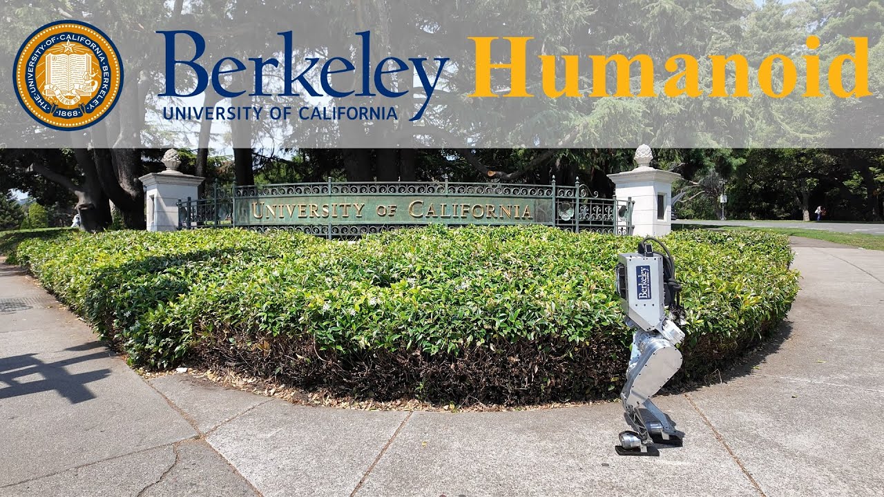
Reinforcement Learning (RL) for bipedal walking is becoming the dominant approach to teach humanoid robots to walk naturally. If you've seen Unitree H1 running at 3.3 m/s or Berkeley Humanoid climbing hills in San Francisco, both were trained with RL — not hand-programmed step sequences.
But why does RL outperform traditional methods? And how do you go from research papers to robots actually walking on the ground? This article dives deep into the full pipeline — from MDP formulation, reward shaping, training in simulation, to sim-to-real transfer.

ZMP vs Reinforcement Learning: Two Different Philosophies
Traditional Approach: ZMP and Model-Based Control
Before RL became popular, humanoid robots walked using the Zero Moment Point (ZMP) method. Core idea: keep the center of pressure (center of pressure) always within the contact area between robot feet and ground (support polygon). Honda ASIMO — the legendary humanoid robot of the 2000s — walked this way.
Problems with ZMP:
- Too conservative: Robot must maintain static balance, so it walks very slowly and rigidly. Humans actually walk by "controlled falling" — continuously losing and regaining balance.
- Not adaptive: Encounters uneven terrain or unexpected pushes easily fail. All trajectories must be pre-calculated.
- Requires accurate models: Any deviation between mathematical model and real robot causes errors.
Reinforcement Learning: Learning from Experience
RL takes a completely different approach: instead of designing controllers by hand, let the robot learn through trial-and-error in simulation. The robot tries millions of steps, receives reward when walking well, penalty when falling — and gradually finds optimal policy.
Result: robots walk more naturally, recover when pushed, adapt to complex terrain, and even run fast — something ZMP-based controllers can hardly do.
The most comprehensive survey paper is Deep Reinforcement Learning for Robotic Bipedal Locomotion: A Brief Survey (Li et al., 2024), summarizing most RL bipedal methods from 2019 to now.
MDP Formulation for Bipedal Walking
To apply RL, first step is modeling the problem as a Markov Decision Process (MDP). This is the most important part — good MDP design determines 80% of success.
Observation Space (State)
What does the robot "see" to decide next action? Observation space typically includes:
# Observation space for bipedal walking policy
observation = {
    # Proprioception — info from internal sensors
    "base_angular_velocity": (3,),    # gyroscope: roll, pitch, yaw rate
    "base_orientation": (3,),         # gravity vector in body frame
    "joint_positions": (12,),         # angles of 12 joints (6 per leg)
    "joint_velocities": (12,),        # joint angular velocities
    "previous_actions": (12,),        # last step's actions

    # Command — desired movement
    "velocity_command": (3,),         # desired vx, vy, yaw_rate
}
# Total: ~45 dimensions
Note: most successful papers don't use vision for locomotion. Only proprioception (joint encoders + IMU). Reason: proprioceptive feedback is high-frequency (1kHz), while cameras only 30-60Hz — too slow for balance control.
Paper Berkeley Humanoid: A Research Platform for Learning-based Control (2024) proves that with simple observation space plus light domain randomization, robots can walk outdoors on complex terrain.
Action Space
Action space determines what the robot controls:
# Action space: target joint positions
action_space = {
    "target_joint_positions": (12,),  # PD target for 12 joints
    # In reality: action = default_pose + policy_output * action_scale
}

# PD controller executes action
torque = kp * (target_position - current_position) - kd * current_velocity
Most common is position targets via PD controller (proportional-derivative). Policy outputs target joint angles, low-level PD controller converts to torque. More stable than outputting torque directly.
Reward Shaping — The Art of Design
This is the hardest part and where researcher experience shows. Reward function determines what behavior robot learns.
def compute_reward(state, action, next_state, command):
    rewards = {}

    # === Tracking rewards (encouraged) ===
    # Reward when velocity matches command
    lin_vel_error = (command.vx - state.base_lin_vel[0])**2
    rewards["linear_velocity"] = math.exp(-lin_vel_error / 0.25) * 1.5

    ang_vel_error = (command.yaw_rate - state.base_ang_vel[2])**2
    rewards["angular_velocity"] = math.exp(-ang_vel_error / 0.25) * 0.5

    # === Regularization rewards (penalized) ===
    # Penalize energy consumption (torque * velocity)
    rewards["energy"] = -0.0001 * torch.sum(
        torch.abs(action * state.joint_velocities)
    )

    # Penalize action change (avoid jerky movements)
    rewards["action_rate"] = -0.01 * torch.sum(
        (action - state.previous_action)**2
    )

    # Penalize excessive body tilt
    rewards["orientation"] = -5.0 * torch.sum(
        state.projected_gravity[:2]**2
    )

    # Reward proper foot contact timing
    rewards["feet_air_time"] = 0.5 * air_time_reward(state)

    # Penalize both feet touching ground too long
    rewards["no_fly"] = -0.25 * both_feet_on_ground(state)

    # Bonus for staying alive
    rewards["alive"] = 2.0

    return sum(rewards.values())
Key insights from papers:
- Exponential reward (form
exp(-error/sigma)) better than linear — smooth gradients and bounded - Feet air time reward critical — without it robot learns to "slide" instead of stepping
- Energy penalty must be small enough not to cancel forward velocity reward, but large enough to prevent wasted movement
Paper Reinforcement Learning for Versatile, Dynamic, and Robust Bipedal Locomotion Control (2024) details reward design for multiple gaits (walking, running, jumping) in one framework.

Training with PPO in Isaac Gym / Isaac Lab
Why PPO?
Proximal Policy Optimization (PPO) is the most popular RL algorithm for locomotion. Reasons:
- Stable: Clipped objective prevents policy updates too large, avoiding "catastrophic forgetting"
- Parallelizes well: Suited for massive parallel simulation on GPU
- Simple: Fewer hyperparameters than SAC or TD3, easier to tune
Original PPO paper: Proximal Policy Optimization Algorithms (Schulman et al., 2017).
Isaac Gym and Isaac Lab
NVIDIA Isaac Gym (and successor Isaac Lab) allows training thousands of robots in parallel on GPU. Game-changer because:
- Speed: 4096 robot instances running simultaneously, collecting experience 1000x faster than single simulation
- GPU-native: Physics runs entirely on GPU, no CPU bottleneck
- Terrain generation: Auto-create complex terrain (stairs, slopes, rocks) for robot learning
Official paper: Isaac Lab: A GPU-Accelerated Simulation Framework for Multi-Modal Robot Learning.
# Example training environment config (Isaac Lab style)
env:
  num_envs: 4096
  episode_length: 1000        # ~20 seconds per episode
  terrain:
    type: "trimesh"
    curriculum: true           # start flat, gradually increase difficulty
    terrain_types:
      - flat: 0.2
      - rough: 0.2
      - slopes: 0.2
      - stairs_up: 0.2
      - stairs_down: 0.2

robot:
  asset: "unitree_h1.urdf"
  default_joint_positions:     # standing pose
    hip_pitch: -0.1
    knee: 0.3
    ankle: -0.2
  pd_gains:
    kp: 100.0
    kd: 5.0

rewards:
  linear_velocity_tracking:
    weight: 1.5
    params: { sigma: 0.25 }
  angular_velocity_tracking:
    weight: 0.5
  energy:
    weight: -0.0001
  action_rate:
    weight: -0.01
  orientation:
    weight: -5.0
  feet_air_time:
    weight: 0.5
  alive:
    weight: 2.0
# Basic training script with Isaac Lab + RSL-RL
from omni.isaac.lab.envs import ManagerBasedRLEnv
from rsl_rl.runners import OnPolicyRunner
# Initialize environment
env = ManagerBasedRLEnv(cfg=HumanoidFlatEnvCfg())
# PPO config
ppo_cfg = {
"algorithm": "PPO",
"num_learning_epochs": 5,
"num_mini_batches": 4,
"clip_param": 0.2, # epsilon in clipped objective
"entropy_coef": 0.01, # encourage exploration
"learning_rate": 3e-4,
"gamma": 0.99, # discount factor
"lam": 0.95, # GAE lambda
"max_grad_norm": 1.0,
"desired_kl": 0.01, # adaptive learning rate
}
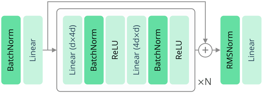
# Policy network: MLP [512, 256, 128]
policy_cfg = {
"actor_hidden_dims": [512, 256, 128],
"critic_hidden_dims": [512, 256, 128],
"activation": "elu",
}
# Train ~2-4 hours on RTX 4090
runner = OnPolicyRunner(env, ppo_cfg, policy_cfg)
runner.learn(num_learning_iterations=5000)
Key open-source framework: legged_gym from ETH Zurich (paper: Learning to Walk in Minutes Using Massively Parallel Deep RL) — basis for most current locomotion research.
Terrain Curriculum
Important technique: curriculum learning for terrain. Instead of throwing robot into hard terrain immediately (learns nothing), start simple then gradually increase difficulty.
# Terrain curriculum: better robot → harder terrain
class TerrainCurriculum:
    def __init__(self):
        self.difficulty_levels = [
            "flat",              # Level 0: flat ground
            "slight_slope",      # Level 1: 5° slope
            "rough_flat",        # Level 2: flat but uneven
            "moderate_slope",    # Level 3: 15° slope
            "stairs_low",        # Level 4: 5cm stairs
            "stairs_high",       # Level 5: 15cm stairs
            "mixed_terrain",     # Level 6: all combined
        ]

    def update(self, success_rate):
        """Level up when robot achieves >80% success rate"""
        if success_rate > 0.8:
            self.current_level = min(
                self.current_level + 1,
                len(self.difficulty_levels) - 1
            )
Sim-to-Real Transfer: Bridge the Reality Gap
Most difficult part of entire pipeline. Robot walks perfectly in simulation but falls immediately on real hardware — the reality gap.
Domain Randomization
Idea: if policy works across many different simulation versions (different friction, mass, delay...), it's also robust on real hardware — which is just "one more version" in the distribution.
# Domain randomization parameters
randomization:
  # Randomize physics
  friction_range: [0.3, 1.5]        # ground friction coefficient
  restitution_range: [0.0, 0.5]     # bounciness
  added_mass_range: [-1.0, 3.0]     # kg added to robot body

  # Randomize robot dynamics
  joint_friction_range: [0.01, 0.15]
  kp_factor_range: [0.8, 1.2]       # ±20% PD gains
  kd_factor_range: [0.8, 1.2]

  # Randomize communication delay
  action_delay_range: [0, 3]         # 0-3 timestep delay
  observation_noise: 0.05            # Gaussian noise sigma

  # Randomize external forces (simulate being pushed)
  push_interval: 8.0                 # seconds
  push_force_range: [0, 100]         # Newtons
Paper Sim-to-Real Transfer in Deep Reinforcement Learning for Bipedal Locomotion (2025) presents combined strategy of domain randomization + curriculum learning + online adaptation — state-of-the-art bipedal sim-to-real.
Additional Techniques
Beyond domain randomization:
- Observation history: Use history of last 5-10 timesteps instead of just current. Helps policy implicitly estimate physical parameters (terrain, friction) without direct measurement.
- Actuator network: Replace ideal PD controller in sim with neural network mimicking real actuator (delay, friction, saturation). Significantly reduces reality gap.
- Teacher-student training: Teacher policy has privileged information access (terrain heightmap, exact friction). Student policy only uses observations available on real robot, distilled from teacher.
Notable Papers and Results
Berkeley Humanoid — Hiking San Francisco
Learning Humanoid Locomotion over Challenging Terrain (Radosavovic et al., 2024) — humanoid robot walking 4+ miles on hiking trail in Berkeley Hills and climbing steepest San Francisco hills. Approach: transformer pre-trained on flat-ground trajectories, then fine-tuned with RL on hard terrain.
Agility Robotics Digit — RL on Commercial Robot
Robust Feedback Motion Policy Design Using RL on a 3D Digit Bipedal Robot — hierarchical RL framework for Digit, combining RL policy with traditional feedback control. Achieves robust walking with reduced state/action space.
Agile and Versatile Bipedal Robot Tracking Control through RL (2024) — small neural network achieving ankle and body trajectory tracking across multiple gaits.
ETH Zurich — Legged Gym Framework
Learning to Walk in Minutes (Rudin et al., 2022) — open-source framework allowing locomotion policy training in minutes on 1 GPU. Foundation for most current research.

Getting Started: Practical Guide
If you want to train a bipedal walking policy yourself, here's the suggested path:
Step 1: Start with MuJoCo + Gymnasium
pip install gymnasium[mujoco]
Try Humanoid-v4 environment. Simplest bipedal problem, sufficient to understand RL pipeline basics.
Step 2: Move to Isaac Lab
# Clone Isaac Lab
git clone https://github.com/isaac-sim/IsaacLab.git
cd IsaacLab

# Install (needs NVIDIA GPU + Isaac Sim)
./isaaclab.sh --install
Isaac Lab provides ready-to-use environments for Unitree H1, G1, and many other humanoids.
Step 3: Customize Reward and Domain Randomization
This is where you'll spend most time. Try changing reward weights, adding/removing reward terms, adjusting domain randomization ranges. Each small change produces very different behavior.
Step 4: Deploy to Hardware (if available)
Unitree G1 (from $16,000) is cheapest platform supporting RL deployment. If no hardware available, many labs offer remote robot access via cloud.
Conclusion
Reinforcement Learning transformed bipedal walking from "nearly impossible" to "train in hours on 1 GPU". Combination of massive parallel simulation (Isaac Lab), stable algorithm (PPO), and sim-to-real techniques (domain randomization, curriculum) creates end-to-end pipeline that anyone with GPU and basic RL knowledge can access.
Humanoid race is heating up — Tesla Optimus, Figure 01, Unitree H1 — and RL is the fuel propelling it forward.