Reinforcement Learning for Robotics — More Than Game Playing
When people think of Reinforcement Learning, they picture AlphaGo or AI playing Atari. But RL for robotics is completely different — robots must interact with real physical world, where every action has consequences (and might break the robot).
In the first part of "AI for Robots" series, I introduce 3 most important RL algorithms for robotics: PPO, SAC, and TD3 — analyzing advantages/disadvantages and guide choosing right algorithm for each problem type.

MDP: Common Language of RL
Before diving into algorithms, understand Markov Decision Process (MDP) — fundamental framework for all RL problems:
- State (s): Current robot state (joint angles, velocities, camera image...)
- Action (a): Action robot takes (torque, velocity command, gripper open/close)
- Reward (r): Feedback signal — did robot perform well?
- Transition (P): How environment changes after action
- Policy (π): Robot's strategy — given state s, which action a?
Example: Robot Arm Grasping
State:  [joint_angles (6D), gripper_pos (3D), object_pos (3D)] = 12D
Action: [joint_velocities (6D), gripper_open/close (1D)] = 7D
Reward: +1 when grasp succeeds, -0.01 per step (encourage speed)
Major differences between RL for games vs robotics:
| Games (Atari, Go) | Robotics | |
|---|---|---|
| Action space | Discrete (up/down/left/right) | Continuous (torque, velocity) |
| State space | Pixels (simple) | High-dimensional (joints + sensors) |
| Safety | Free resets | Breaking robot costs money |
| Sample efficiency | Millions of steps fast | Each step takes real time |
| Reward | Dense (score increases) | Sparse (only +1 on success) |
These characteristics determine algorithm choice — and why not every algorithm is suitable for robots.
PPO: On-Policy, Stable, Most Popular
Proximal Policy Optimization (PPO) (Schulman et al., 2017) is the most common RL algorithm in robotics today. From OpenAI Five to locomotion policies in research labs, PPO is the default choice.
How It Works
PPO belongs to the policy gradient family — directly optimizes policy using gradient ascent. Key innovation: limit policy change per update with clipped objective, ensuring stability critical for robots:
L_CLIP = E[min(r(θ) × A, clip(r(θ), 1-ε, 1+ε) × A)]

r(θ) = π_new(a|s) / π_old(a|s)   // probability ratio
A = advantage estimate              // how much better than average
ε = 0.2 (commonly used)            // change limit
This ensures policy doesn't change too much each update — very important for robots because sudden changes can cause instability.
Advantages
- Stable: Rarely diverges even with imperfect hyperparameters
- Simple to implement: Compared to TRPO (requires Hessian), PPO uses standard gradients
- Parallelizable: Collect data from many environments simultaneously
- Works with both discrete and continuous actions
Disadvantages
- Sample inefficient: Needs millions of steps because on-policy (uses data once then discards)
- Not for real robots: Too many samples = too many real robot hours
- Hyperparameter sensitive for some tasks
When to Use PPO?
PPO is top choice for:
- Locomotion (walking, running, jumping) — dense reward, trainable in simulation
- Sim-to-real — train millions of steps in sim, transfer to real robot
- Multi-agent — many robots learning simultaneously
SAC: Off-Policy, Sample Efficient, Continuous
Soft Actor-Critic (SAC) (Haarnoja et al., 2018) is the answer to PPO's sample efficiency problem. SAC is off-policy — can reuse old data, greatly reducing samples needed.
How It Works
SAC optimizes maximum entropy objective — doesn't just maximize reward but also maximizes policy entropy (diversity):
J(π) = E[Σ γ^t (r(s_t, a_t) + α × H(π(·|s_t)))]

H(π) = -E[log π(a|s)]   // policy entropy
α = temperature           // balance reward vs exploration
The entropy bonus makes the robot not just learn one way but learn many approaches — if the primary method fails, there are backups. Very important for manipulation where environment changes.
Advantages
- Sample efficient: Off-policy, replay buffer — reuse old data many times
- Stable training: Entropy regularization + dual Q-networks
- Continuous actions: Specifically designed for continuous action space (robot joints)
- Automatic temperature tuning: Automatically adjusts alpha
Disadvantages
- More complex than PPO: 5 networks (2 Q, 2 Q-target, 1 policy)
- No discrete actions (original version)
- Replay buffer uses memory: Stores all transitions
When to Use SAC?
SAC is ideal for:
- Manipulation (grasping, placing, assembly) — sample efficiency matters
- Training on real robot — each sample is precious, cannot waste
- Continuous control — robot arms, grippers
TD3: Off-Policy, Addresses Overestimation
Twin Delayed DDPG (TD3) (Fujimoto et al., 2018) is an improved version of DDPG, solving Q-value overestimation — when the model overestimates action values, leading to poor policy.
Three Key Techniques
- Twin Q-networks: Use 2 Q-networks, take the minimum to reduce overestimation
- Delayed policy update: Only update policy every 2 Q-updates (reduces error propagation)
- Target policy smoothing: Add noise to target actions (regularization)
# TD3 core: take min of 2 Q-networks
Q_target = reward + gamma * min(Q1_target(s_next, a_next), Q2_target(s_next, a_next))
# a_next = policy_target(s_next) + clipped_noise
Quick Comparison: TD3 vs SAC
| TD3 | SAC | |
|---|---|---|
| Policy | Deterministic | Stochastic |
| Exploration | Manual noise addition | Entropy bonus automatic |
| Multi-modal | No | Yes |
| Tuning | Simpler | Alpha automatic but more complex |
Comprehensive Comparison Table
| Criterion | PPO | SAC | TD3 |
|---|---|---|---|
| On/Off-policy | On-policy | Off-policy | Off-policy |
| Sample efficiency | Low | High | High |
| Training stability | Very high | High | Medium |
| Continuous actions | Yes | Yes (best) | Yes |
| Discrete actions | Yes | No (original) | No |
| Hyperparameter sensitivity | Low | Medium | Medium |
| Multi-modal policy | Yes (stochastic) | Yes (stochastic) | No (deterministic) |
| Memory usage | Low | High (replay buffer) | High (replay buffer) |
| Implementation complexity | Simple | Complex | Medium |
| Best for | Locomotion, sim | Manipulation | Simple control |

Algorithm Selection Guide
Simple flowchart for choosing algorithm:
- Does the problem have discrete actions? → Use PPO
- Can you train in simulation? → Use PPO (millions of steps free)
- Must train on real robot? → Use SAC (most sample efficient)
- Manipulation with continuous control? → Use SAC
- Need simple baseline? → Use TD3
In practice, PPO for locomotion and SAC for manipulation is the most common combo in robotics labs.
Hands-On: Train PPO with Stable Baselines3
Let's start with a simple example — train a biped robot to walk using PPO. Stable Baselines3 is the most popular RL library, wrapping algorithms into easy-to-use API.
"""
Train PPO for BipedalWalker — 2-legged robot learning to walk
Requires: pip install stable-baselines3[extra] gymnasium
"""
import gymnasium as gym
from stable_baselines3 import PPO
from stable_baselines3.common.env_util import make_vec_env
from stable_baselines3.common.callbacks import EvalCallback

# 1. Create environments — 8 parallel to increase sample speed
env = make_vec_env("BipedalWalker-v3", n_envs=8)
eval_env = make_vec_env("BipedalWalker-v3", n_envs=1)

# 2. Initialize PPO with good hyperparameters for locomotion
model = PPO(
    policy="MlpPolicy",
    env=env,
    learning_rate=3e-4,
    n_steps=2048,           # Steps per env before each update
    batch_size=64,
    n_epochs=10,            # Iterations through data each update
    gamma=0.99,             # Discount factor
    gae_lambda=0.95,        # GAE lambda for advantage estimation
    clip_range=0.2,         # PPO clip range (epsilon)
    ent_coef=0.01,          # Entropy bonus — encourages exploration
    verbose=1,
    tensorboard_log="./logs/ppo_bipedal/",
)

# 3. Callback to evaluate and save best model
eval_callback = EvalCallback(
    eval_env,
    best_model_save_path="./models/ppo_bipedal/",
    log_path="./logs/ppo_bipedal/",
    eval_freq=10000,        # Evaluate every 10K steps
    deterministic=True,
    render=False,
)

# 4. Train! BipedalWalker needs ~1-2 million steps to converge
model.learn(
    total_timesteps=2_000_000,
    callback=eval_callback,
    progress_bar=True,
)

# 5. Test trained model
model = PPO.load("./models/ppo_bipedal/best_model")
env = gym.make("BipedalWalker-v3", render_mode="human")

obs, _ = env.reset()
total_reward = 0

for _ in range(1000):
    action, _ = model.predict(obs, deterministic=True)
    obs, reward, terminated, truncated, info = env.step(action)
    total_reward += reward

    if terminated or truncated:
        print(f"Episode reward: {total_reward:.1f}")
        obs, _ = env.reset()
        total_reward = 0

env.close()
Key Hyperparameter Explanations
| Parameter | Value | Meaning |
|---|---|---|
n_steps |
2048 | Steps collected before each update. Large = more stable, small = faster |
n_epochs |
10 | Iterations through data. PPO allows many epochs thanks to clipping |
clip_range |
0.2 | Policy change limit. 0.1-0.3 usually works well |
ent_coef |
0.01 | Entropy bonus. Increase if robot doesn't explore enough |
gae_lambda |
0.95 | Bias-variance tradeoff for advantage. 1.0 = low bias, 0.0 = low variance |
Training Tips for Robot RL
- Always start in simulation: Isaac Gym, MuJoCo, PyBullet — train 1000x faster than real
- Reward shaping is critical: Sparse reward (+1 on completion) rarely works alone. Add intermediate rewards (distance to target, correct direction...)
- Normalize observations: Robot sensors have different ranges — normalize to [-1, 1]
- Log everything: TensorBoard is best friend when debugging RL
Next Steps
RL is the foundation, but for many manipulation tasks, imitation learning is far more practical — especially when you have human demonstrations available. In the next post, Imitation Learning: BC, DAgger and DAPG for Robots — methods for learning directly from demonstrations.
For locomotion applications: RL for Bipedal Walking: From Simulation to Real Robot
Related Articles
- Imitation Learning: BC, DAgger and DAPG for Robot — Part 2 of AI for Robot series
- RL for Bipedal Walking: Simulation to Real Robot — Applying PPO to biped robots
- Sim-to-Real Transfer: Train Simulation, Run Real Robot — Transfer model from sim to real robot
- Foundation Models for Robot: RT-2, Octo, OpenVLA — Latest trends in robot AI